Showing posts with label Biometrics Open Access Journal. Show all posts

Monday, 27 June 2022

Lupine Publishers| The Gompertz Length Biased Exponential Distribution and its application to Uncensored Data

 Lupine Publishers| Journal of Biostatistics & Biometrics


Abstract

This paper proposes a generalization of the length biased exponential distribution, called the Gompertz length biased exponential (GLBE) distribution. Some of the basic properties of the proposed model were derived in minute details and model parameters estimated by the maximum likelihood estimate method. The adequacy of the model is empirically validated with the use of real - life data.

Keywords: Exponential Distribution; Length Biased; Gompertz Generalized Family Of Distribution; Quantile Function; Hazard Functions; Survival Function

Introduction

Length biased distributions are special case of the more general form known as weighted distribution [1], first introduced by [2] to model ascertainment bias and formalized in a unifying theory by [3]. Lifetime data may be modeled with several existing distributions, although the existing models are not adequate or are less representative of actual data in many situations. Therefore, the development of compound distributions that could better describe certain phenomena and make them more flexible than the baseline distribution is of great importance [4]. Thus, the choice of the model is also an important issue for reliable model parameter estimation. Some exponential distribution generalizations for modeling lifetime data due to some interesting advantages have been recently proposed [5]. In recent years many exponential distribution generalizations have been developed, such as the Marshall Olkin length biased exponential distribution [5], exponentiated exponential [6,7], generalized exponentiated moment exponential [8], extended exponentiated exponential [19], Marshall-Olkin exponential Weibull [10], Marshall-Olkin generalized exponential [5], and exponentiated moment exponential [11] distributions.

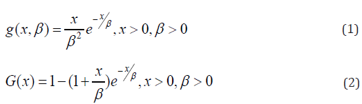
A random variable X is said to have a length biased exponential distribution with parameter \beta if its probability density function (pdf) and cumulative distribution function (cdf) is given by equation (1) and (2) respectively [12]:

Lupinepublishers-openaccess-Biostatistics-Biometrics-journal

Where is the scale parameter.

The survival function is given by the equation

Lupinepublishers-openaccess-Biostatistics-Biometrics-journal

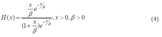
The hazard function is

Lupinepublishers-openaccess-Biostatistics-Biometrics-journal

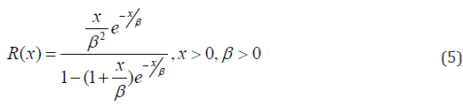
And the reversed hazard rate function is

Lupinepublishers-openaccess-Biostatistics-Biometrics-journal

Alzaatreh et al. [13] defined the cumulative distribution function of the Transformed-Transformer (T-X) family of distributions by;

Lupinepublishers-openaccess-Biostatistics-Biometrics-journal

And the corresponding probability density function by;

Lupinepublishers-openaccess-Biostatistics-Biometrics-journal

Morad Alizadeh et al [14] defined the cumulative distribution function and probability density function of the Gompertz Generalized family of distribution by setting

Lupinepublishers-openaccess-Biostatistics-Biometrics-journal

respectively. Where \theta and \gamma are additional shape parameters whose role is to vary the tail length.

Thus, we proposed a new generalization of the length biased exponential distribution called the Gompertz length biased exponential (Go-LBE) distribution. In the rest of the paper, we define the Go-LBE model and plots for different parameter values in Section 2; some of the statistical properties of the proposed Go-LBE distribution are discussed in minute details in section 3, Application of the Go-LBE distribution to a lifetime data in section 4. The concluding remark is presented in section 5.

Gompertz Length Biased Exponential (Go-LBE) Distribution

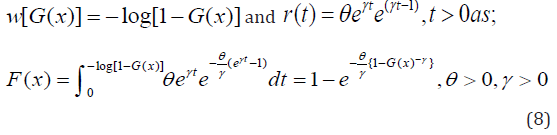
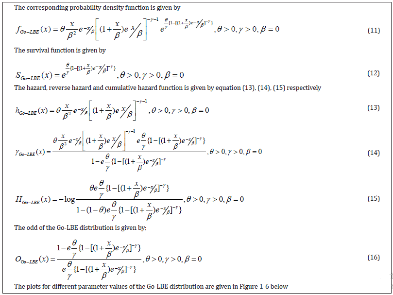
The cumulative distribution function of the

Lupinepublishers-openaccess-Biostatistics-Biometrics-journal

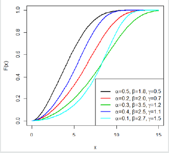
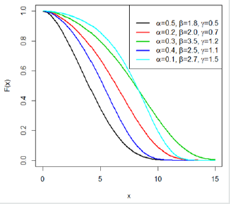
Figure 1: Graph for Go-LBE cumulative distribution function at different parameter values.

Lupinepublishers-openaccess-Biostatistics-Biometrics-journal

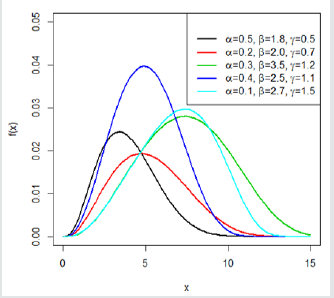
Figure 2: Graph for Go-LBE probability density function at different parameter values.

Lupinepublishers-openaccess-Biostatistics-Biometrics-journal

Figure 3: Graph for Go-LBE survival function at different parameter values.

Lupinepublishers-openaccess-Biostatistics-Biometrics-journal

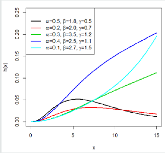
Figure 4: Graph for Go-LBE hazard function at different parameter values.

Lupinepublishers-openaccess-Biostatistics-Biometrics-journal

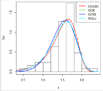
Figure 5: Histogram of the fitted distributions.

Lupinepublishers-openaccess-Biostatistics-Biometrics-journal

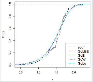
Figure 6: Empirical cdf of the fitted distributions.

Lupinepublishers-openaccess-Biostatistics-Biometrics-journal

Some Statistical Properties of the Go-LBE Distribution

Basic properties such as the asymptotic behavior, parameter estimation and order statistics of the Go-LBE distribution are discussed in minute details.

Asymptotic Behavior

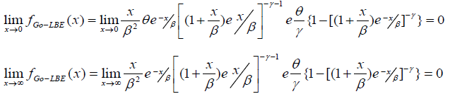
Here we critically examine the behavior of the Go-LBE model in equation (11) as x→0 and as x→∞

This indicates that the Gompertz length biased exponential distribution is unimodal. A clear observation of Figure 2 shows the Go-LBE model has only one peak. This supports our claim that the Go-LBE distribution has only one mode.

Parameter Estimation

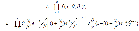
Using maximum likelihood estimation techniques, we estimate the unknown parameter of the Go-LBE model based on a complete sample. Let X...Xn indicate a random sample of the complete Go-LBE distribution data, and then the sample’s likelihood function is given as;

We can now express the log likelihood function as;

Lupinepublishers-openaccess-Biostatistics-Biometrics-journal

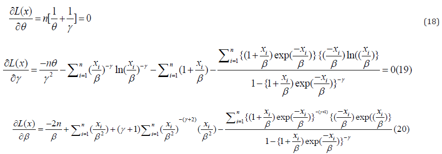
By taking the derivative with respect toθ ,γ andβ , and fixing the outcome to zero, we have;

Lupinepublishers-openaccess-Biostatistics-Biometrics-journal

Solving equation (18)-(20) iteratively, will give the estimate of the parameters of the Go-LBE model.

Order Statistics

We considered a random sample denoted by from the densities of the Go-LBE distribution. Then,

The probability density function of the order statistics for the Go-LBE distribution is given as;

Lupinepublishers-openaccess-Biostatistics-Biometrics-journal

The Go-LBE distribution has minimum order statistics given as;

Data Analysis

Here, we provide an application of the Gompertz length biased exponential distribution by comparing the results of the model fit with that of other Gompertz- G family of distributions. The data set we employ is the uncensored strength of 1.5cm glass fibre data previously used by Bourguignon M et al. [15], Merovci F et al. [16]. This data set will be used to compare between fits of the Gompertz length biased exponential distribution (Go-LBE) with that of Gompertz-Exponential (Go-E), Gompertz-Lomax (Go-L), and, Gompertz-Weibull (Go-W). The data is presented below (Tables 1 & 2):

Table 1: Descriptive Statistics on Cancer Stem Cell Data.

Lupinepublishers-openaccess-Biostatistics-Biometrics-journal

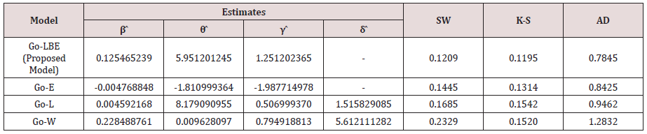
Table 2: MLEs, SW, AD and K–S of parameters for Cancer Stem Cell data.

Lupinepublishers-openaccess-Biostatistics-Biometrics-journal

0.55, 0.74, 0.77, 0.81, 0.84, 1.24, 0.93, 1.04, 1.11, 1.13, 1.30, 1.25, 1.27, 1.28, 1.29, 1.48, 1.36, 1.39, 1.42, 1.48, 1.51, 1.49, 1.49, 1.50, 1.50, 1.55, 1.52, 1.53, 1.54, 1.55, 1.61, 1.58, 1.59, 1.60, 1.61, 1.63, 1.61, 1.61, 1.62, 1.62, 1.67, 1.64, 1.66, 1.66, 1.66, 1.70, 1.68, 1.68, 1.69, 1.70, 1.78, 1.73, 1.76, 1.76, 1.77, 1.89, 1.81, 1.82, 1.84, 1.84, 2.00, 2.01, 2.24

For all competing distributions using the strength of glass fibre data set, Table 2 shows parameter estimate and the value for the Shapiro Wilk (S-W), Anderson Darling (AD), and the Kolmogorov Smirnov (K-S) statistic (Table 3).

From Table 3, the Go-LBE has the highest log-likelihood values and the lowest AIC, CAIC, BIC and HQIC values; hence, it is chosen as the most appropriate model amongst the considered distributions.

Table 3: Log-likelihood, AIC, AICC, BIC and HQIC values of models fitted for Cancer Stem Cell data.

Lupinepublishers-openaccess-Biostatistics-Biometrics-journal

Conclusion

This research has successfully extended the length biased exponential distribution. Densities and basic statistical expressions were briefly derived. The performance of the proposed Gompertz length biased exponential distribution was compared to existing models in literature based on the negative log likelihood, AIC, CAIC, BIC and HQIC values. Based on the lowest criterion values, we therefore conclude that the Gompertz length biased exponential distribution is the most suitable model amongst the considered models and indeed a very competent model for describing life-time situations.

Read More About Lupine Publishers Journal of Biostatistics & Biometrics Please Click on Below Link: https://lupine-publishers-biostatistics.blogspot.com/

Tuesday, 16 November 2021

Lupine Publishers| Demand for the Emerging AI, Machine, Deep Learning and Big Data Analytics Skill for 21st Century Jobs

 Lupine Publishers| Journal of Biostatistics & Biometrics


Abstract

This paper presents recent development, application and potentials of technologies like AI, Machine, Deep Learning and Big Data Analytics and ways in which big data can be leveraged to improve the efficiency and effectiveness of government. It describes the demand of skills for handling of massive and diverse sets of information that are gathered, processed, and analyzed for scientific discovery. Job prospect are also highlighted.

Introduction

Data generation is presently is light-years ahead compared to where it was a few years ago. With technological advances and use, huge digital information is now available that is beyond our imagination. It is widely accepted that Big data analytics has revolutionized digital transformation. It enables too quick and indepth analysis, facilitating faster accurate decisions resulting in right insight. In fact, technological advances in data management have helped in timely capture of the informational value of big data. As a result, a wide adoption of analytics has happened that were not economically viable for large-scale applications before the big data era. Importantly, Pet bytes of raw data provide lot of clues for health care services through right use. Data is considered as gold in digital economy era. It is needless to mention that today analytics skills are extremely in high demand. A wide gap has been created in demand and supply of analysts throughout the globe particularly in western countries. According to the experts in the field knowledge of data analytics is essential for this next generation job aspirants. Now we are in the age of data. Everybody talks about big data across all the fields of science and technology. Even Big data analytics is attempted in the non-conventional areas. It is considered as a “the next big thing” will be. Now a day’s data is generated in higher quantities from various field and analyzed at a faster and with higher accuracy that we could not have thought of a few years ago. Researchers adding every day, new tool to extract raw data into valuable insight enabling solutions to the critical problems. The application of big data is enormous in all spheres of scientific investigation. Technologies coupled with and internet of things produces huge data globally. Innovative technologies have added capacity to generate, store, and analyze data from different sources for a various application. Some 2.5 quintillion bytes of data are produced every day, and approximately 90 percent of existing data was produced in the last two years alone [1]. These data are the potential sources for innovative research.

Are we ready to embrace Big Data? It is time to think whether we are capable to make use of big data’s potential? Of course, success will obviously require new skills and new perspectives particularly for potentially disruptive business models [2]. New development in the areas of big data expands the suitable space for development of algorithms, AI and machine-mediated analysis. Companies that exploit the data are the ones turning data into gold. With the right aptitude in analyzing IoT data, one can make internal business changes to turn data into revenue by marketing insights which are in high demand [3]. Knowledge and Skill Requirement: Data without domain knowledge are just facts and numbers. Curiosity and passion are essential data analysts. One must accept that presently data is available, but knowledge is not only scarce but expensive too. Therefore, the lies the demand for Data Scientists with the skill and the mind-set to apply Big Data technologies in right perspective.

Application in Science and Technology

In the last five years, more scientific data has been generated than in the entire history of mankind. Now one can imagine what is going to happen in the next five. Genetics and proteomics generate high-dimensional data in scale. In big data lies the potential for revolutionizing in the nonconventional areas like Police employing seismology-like data models to predict and check crimes. Astronomers using the Kepler telescope snag information on 200,000 stars every 30 seconds, which has led to the discovery of the first Earth-like planets outside our solar system. Businesses are switching over to social networking data for higher return. The same phenomena are true for public health. DNA sequencing has held big data’s starring role, as a single human genome consists of some 3 billion base pairs of DNAs. Human genome’s right analysis gives clues to infections, cancer, and production processes, customers and markets [4].

Real Time Analytics

As per latest information the NASA’s Mars Rover spacecraft resorted to Big Data driven analytical engines for discovery. The Elastic search technology being open source is utilized by Netflix and Goldman Sachs. NASA’s Jet Propulsion Lab’s mission has now rebuilt its analytics systems around an Elastic search that processes all the data transmitted from the Rover during its four daily scheduled uploads runs the day-to-day mission planning [5]. Role of Big data for pollution control. Interestingly, with the aid of sensors laid on roads take stock of the total emissions that traffic discharge during the day. The data is used to coordinate with the traffic police. Traffic data processing helps management for planned diversion through the less congested areas to minimize carbon emissions in target areas [6]. Recent development in the areas of Computer Science, the Big Data is booming as can be evidenced from its use by Fortune 1000 companies resulting in quick, financial growth for startups. According to the World Economic Forum Most Innovative Startups In the world are Diagnostics, Sweden; Agrosmart, Brazil, Appeal Sciences, USA; Applied Brain Research, Canada; Aqua Security, Israel; Armis, USA; Benevolent, UK; Best mile, Switzerland and many more. Every year, thousands of new companies aim on becoming the next big success story with innovative products, efficient operations and strong leadership and these companies are likely to shape the future.

Artificial intelligence (AI) is a hot topic now. AI these days are taking off as data availability is not a problem in the current digitized. As we know. Machine learning is used to develop predictive models by identifying patterns from huge datasets. Predictive data analytics applications are in wide use for price prediction, risk assessment, and predicting customer behavior. Machine learning provides computer science that gives computers the ability to learn without being explicitly programmed. It is in fact; deep learning is the main driver and the most important approach to AI. It may be noted that as per the industry-watchers many of the companies listed are utilizing artificial intelligence, as well as a number of biotech firms and block chain technologies. New technologies like machine learning and artificial intelligence are used by researchers for innovation. Technology giants such as Google, Apple, IBM, Face book and many more are investing heavily for extracting intelligence. So, need of the hour is to acquire knowledge in the areas of Artificial Intelligence, deep learning, machine learning, to keep pace with industry requirements. Undoubtedly, data analysis is not simple that requires both human and machine’s working in coordination.

Job Prospect

According to the survey report, repetitive jobs are most likely to be taken over by Artificial Intelligence (AI) in future like BPO, manual testing, system maintenance and infrastructure management etc. A survey reveals that Big Data and Data Science, Big Data Architect, Big Data Engineer, Artificial Intelligence and IoT Architect, and Cloud Architect as the job will be high in demand in the near future. The demand for people with the deep analytical skills in big data including machine learning and advanced statistical analysis are very high.. As many as 140,000 to 190,000 additional specialists may be required in addition to 1.5 million managers and analysts with knowledge and understanding of application of big data in real data life. Companies may take care of their recruitment and retention programs, along with training of key data personnel. The greater access to personal information that big data often demands will place a spotlight on another tension, between privacy and convenience. According to Peter Fader “The real beauty of analytics is not just collecting a lot of data, but it’s finding out ways to do it in a systematic manner”. According to the survey report, the jobs that are in the jeopardy of getting extinct are the ones that have become repetitive and are most likely to be taken over by Artificial Intelligence (AI) in next five years or so. These include job profiles such as BPO, manual testing, system maintenance and infrastructure management etc. The greater access to personal information that big data often demands will place a spotlight on another tension, between privacy and convenience.

Conclusion

As per latest estimate, a reported 3.2 billion Internet users and over 4.6 billion of mobile phones users are regularly generating huge data through communication [7] and the number is increasing day by day. Within these data lies a lot of valuable information. Now it is the job of data scientists and analysts to extract knowledge out of the same. Here lies the demand for skilled manpower to execute the task using right tools and techniques for analytical insights. Literature on tools and techniques for handling these areas are covered [8]. Utmost care is needed towards data privacy issue as well.

Read More Lupine Publishers Journal of Biostatistics & Biometrics Please Click on Below:
https://lupine-publishers-biostatistics.blogspot.com/

Tuesday, 24 August 2021

Lupine Publishers| Correlative Variation of The Essential Amino Acids

 Lupine Publishers| Current Trends on Biostatistics & Biometrics (CTBB)


Abstract

On the example of the table of contents of eight essential amino acids in 22 products, the methodology of factor analysis and determination of the coefficient of correlation variation, calculated as the ratio of the sum of the correlation coefficients of stable laws and laws of binary relations between amino acids to the product of the number of amino acids as influencing variables and as dependent indicators. It is shown that this evaluation criterion depends on the composition of the products and the set of amino acids considered. Therefore, it is proposed to make a more complete table considering the set of objects, which considers the content of all 20 amino acids. The law of binary relations between amino acids is the sum of the exponential law and the biotechnical law of stress excitation in the product. By correlation coefficients of individual binary relations, the ratings of amino acids as influencing variables and as dependent indicators are performed. The correlation matrix of super strong bonds of essential amino acids with correlation coefficients of more than 0.99 is considered, in part of which the graphs are given. By the nature of behavior, it is proposed to classify the binary relationships between amino acids into positive, neutral and negative. Separately, the method of rating products. The equations and graphs of rank distributions of the content of essential amino acids in products are given. The rating of essential amino acids by dispersion of residues from the equations of binary relations and rank distributions is given.

Keywords: Amino Acids; Products; Factor Analysis; Regularities; Correlation Coefficients; Coefficient of A Correlative Variation

Introduction

Under the expression correlative variation Charles Darwin understands that the whole organization is internally connected during growth and development, and when weak variations occur in one part and are cumulated by natural selection, the other parts are modified. Modifications in the structure recognized by taxonomists for a very important, can depend solely on the laws of variation and correlation [1]. For example, Phyto enosis [2] has at least three fundamental properties: first, the correlative variation in the values of parameters in time and space; second, the correlation depends on the genotypic properties of the plant species; third, the variation is due to phenotypic properties, as well as the cycles of solar activity [3], the rotation of the moon around the Earth and our planet around itself [4].

In accordance with the correlative variation of Charles Darwin, during the growth and development of the body, significant changes in the initial age will lead to changes in the structure and in the adult creature. Therefore, people, taking, and thereby enhancing some feature of, almost, probably, unintentionally modifying other parts of the body based on the mysterious laws of correlation [1]. Any non-investigative variation is insignificant for us. But the number and variety of hereditary deviations in the structure, both minor and very important in physiological terms, is infinite. All things are things, properties and relations [5], and in the bios relations control things and change their structures. The purpose of the article is to show the laws and regularities of the correlative variation of the content of eight essential amino acids in a set of 22 products.

The Concept of Correlative Variation

Variability [1] is usually associated with the living conditions that the species has been subjected to for several successive generations. In General, according to Darwin, there are two factors: the nature of the body (most important factor) and the properties of existing conditions [1]. Thus, we adopted the basic hypothesis that typing, and the classification has no effect on biotech based on mastery of life laws. Therefore, the variation (the set of deviations from the Darwin correlation) depends on the human factor, i.e. on the quality of measurements of soil properties and plants [4,6]. Soil according to V.V. Dokuchaev [7] is a living organism. Therefore, the principle of Darwin’s correlative variation should provide high adequacy of the revealed regularities [6]. Similarly, a priori we will consider experiments with essential amino acids [8] to measure their concentration in different types of products for humans and animals highly correlative.

From the concept of correlative variation of Charles Darwin, which was not understood by mathematicians and was not developed by biologists, it clearly follows that in other conditions of the habitat other combinations of values of factors may be stronger (Darwin calls factors hereditary deviations). Therefore, weak factor connections may be stronger for other combinations of the studied objects. As a result, there is a mathematical tool [9- 12] (identification method) for comparison of different natural and artificial (technical) objects [13]. The coefficient of correlative variation is considered for many factors of the physical object of study, that is, biological, chemical, technological, socio-economic, etc. It is equal to the ratio of the total sum of the correlation coefficients to the square of the number of factors for the complete table model (or to the product of the number of factors and). The type of the system under study does not affect this criterion, and the correlation variation depends entirely on the internal properties of the system under study. The coefficient of correlative variation is calculated by the formula

Lupinepublishers-openaccess-Biostatistics-Biometrics-journal

where

K – the coefficient of correlative variation of the set of factors or parameters characterizing the system under study,

ΣΣr – the total sum of the correlation coefficients for the rows and columns of the correlation matrix of the relationships between the factors,

N – number of factors to consider in the symmetric table,

Nx, Ny – the number of factors on the axes x and y .

Functional connectivity is a universal property of matter. For example, internal correlation variation is observed in the results of agrochemical analysis of soil samples [6], as all agrochemical parameters are measured on the same sample. Sampling sites do not affect the internal connectivity of biochemical and other reactions, that is, the same interactions between chemical elements and their compounds are observed on Earth. Such a community is called an ecosystem [2] or a biosphere superposition. The strongest correlative variation over 0.999 is observed in the set of genes [13- 15]. Slightly less, but more than 0.99, as will be shown in this article, such a variation exists in the group of essential amino acids.

Essential Amino Acids

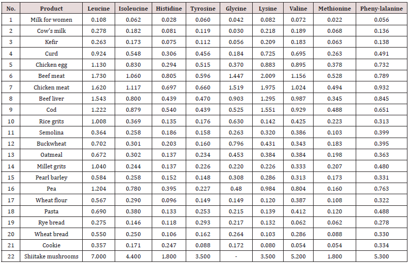
These are essential amino acids for animals that cannot be synthesized in the body, in particular, human. Therefore, their intake from food is necessary (Table 1).

Table 1: The content of essential amino acids in products [1] (grams per 100 grams of product), We have included in the list of products №22 «Shiitake mushrooms».

Lupinepublishers-openaccess-Biostatistics-Biometrics-journal

Rating of Influencing and Dependent Factors

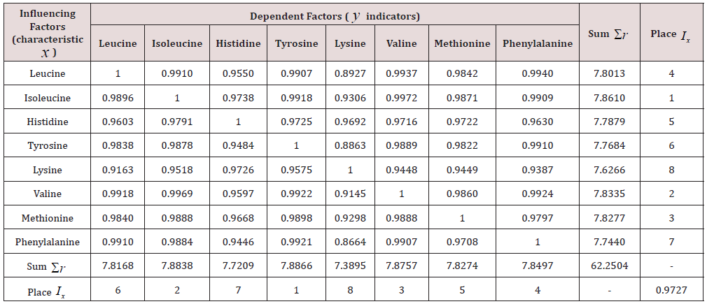
To determine the coefficient of correlative variation of nine amino acids among 22 types of products it is necessary to conduct a factor analysis [9]. Due to the absence of a measured value of glycine content in one cell of Table 1 in the row Shiitaki mushrooms, factor analysis was first carried out [9, pp. 82-83, table. 3.30] nine factors and 21 products. The coefficient of correlative variation was equal to 0.9985. All binary 92– 9 = 72 relations are characterized by the exponential law. Table 2 shows the correlation matrix of binary relationships and the rating of eight factors excluding glycine for 22 products according to Table 1.

Table 2: Correlation matrix of factor analysis without glycine and rating of factors in identification by the exponential law.

Lupinepublishers-openaccess-Biostatistics-Biometrics-journal

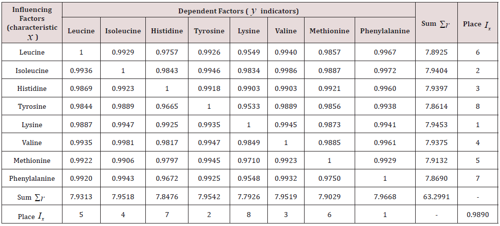
Table 3: Correlation matrix of factor analysis without glycine and rating of factors in identification by exponential and biotechnical law.

Lupinepublishers-openaccess-Biostatistics-Biometrics-journal

Table 3.1:

Lupinepublishers-openaccess-Biostatistics-Biometrics-journal

The coefficient of correlative variation is 0.9727, which is significantly less than 0.9985. In the future, it turned out that in addition to the indicative law, the biotechnical law [4,6,9-15] of the stress excitation of amino acids depending on each other is additionally considered (Table 3). With the coefficient of correlative variation 0.9890 in the first place among the influencing variables was lysine, and among the indicators -phenylalanine. Thus, the correlative variation is very sensitive to the composition of amino acids and products. This fact in the future will reveal the rational compositions, structures and functions of amino acids in different systems under study.

The Law of the Relationship Between Amino Acids

It is expressed by an equation of the form

Lupinepublishers-openaccess-Biostatistics-Biometrics-journal

where y- amino acid content in the product as an indicator (g per 100 g of product),

x- amino acid content of the product as an influencing variable (g per 100 g of product),

a1..... a6 - the parameters of the model (2) taking the numerical values in the course of structural-parametric identification in the software environment CurveExpert-1.40. Formula (2) shows three types of stress-induced amino acids under the influence of each other: positive, neutral and negative. Neutral type appears only without shiitake mushrooms, that is, when the amino acid content changes from 0 to 2 (maximum 2.009 for beef). The maximum concentrations of nine amino acids without shiitaki mushrooms are in two products-beef and chicken meat. In the amino acid content range from 2 to 7 in Table 1 there are no types of products (except mushrooms). Therefore, it is necessary to add new products to the list and Table 1.

In the concentration range from 0 to 7, two types of behavior appear:

  1. positive behavior, with a positive sign in front of the second component of the formula (2), when with increasing content of the influencing amino acid, the content of the dependent amino acid increases according to the biotechnical law of stress excitation;
  2. negative behavior, with a negative sign, when the content of the dependent amino acid is inhibited from the action of the wagging amino acid. These two types provide optima for the interaction of essential amino acids.

Conclusion

We have extended the principle of correlative variation not only to Charles Darwin organisms, but also to populations (in the article population of eight amino acids) and even to any biological, biotechnical and technical systems [13]. This principle allows to compare heterogeneous systems on one or some set of factors by functional connectivity. The coefficient of correlative variation, as a generalized criterion for comparing different sets of homogeneous biological objects, gets a very high value. For example, populations of genes [14,15] obtained the correlative coefficient of variation not less than 0.9999. In the example of this article, the level of adequacy for the set of eight essential amino acids is not less than 0.99. This makes it possible in the future to create the most complete table of contents and other indicators for a system of 20 amino acids and hundreds of objects, including products. Functional connectivity between essential amino acids was super strong and it is subject to a simple formula of two-term trend containing exponential and biotechnical laws. The absence of the second term determines the neutral type of behavior, and signs in the presence of the second member characterize the positive (+) or negative (-) type of behavior of amino acids in the studied system of products. To identify the effect of oscillatory adaptation of essential amino acids to each other in some sets of products need more accurate (with measurement error, less than an order of magnitude) data.

Read More About Lupine Publishers Current Trends on Biostatistics & Biometrics (CTBB) Please Click on Below Link:  https://lupine-publishers-biostatistics.blogspot.com/

Tuesday, 29 June 2021

Lupine Publishers| Phenotypic Correlation Between Egg Weight and Egg Linear Measurements of the French Broiler Guinea Fowl Raised in the Humid Zone of Nigeria

 Lupine Publishers| Current Trends on Biostatistics & Biometrics (CTBB)


Abstract

This study was carried out in Funtua, Kastina State. A total of 119 Eggs of the French broiler guinea fowl were sourced at Songhai Agricultural center Funtua, Kastina State. The eggs were measured for egg linear measurements and egg length and egg width. Data obtained was subjected to statistical package for analysis [1]. The correlations between body weight and body linear measurements were determined using pearsons product moment correlation coefficient (r). Phenotypic correlation between egg weight and egg linear measurements was also determined. Egg weight had positive and significant (P<0.05) correlation with egg length (0.275) and egg width (0.496). The correlation between egg shell index was negative (-0.058). The result shows that Egg weight can be improved by selection for egg length and width French broiler guinea fowl populations.

Keywords: Broiler-Guinea-Fowl; Correlation; Egg Linear Measurement; Egg-Weight

Introduction

Meat and meat products are major sources of high-quality protein and their amino acid composition usually compensates for deficiencies in the staple foods. Production of family poultry is regarded as an alternative way to alleviate poverty and support to ensure food security for socio-economically disadvantaged rural households (Branckaert and Gue’ye, 1999). In third world countries, the guinea fowl production could become much more valuable than it is today (Siana, 2005; Fajmilehin, 2010; Moreki, 2010). It thrives under semi intensive and extensive conditions, forages well, and requires little attention from the farmer (Dahauda, 2007). The guinea fowl also retains many of its wild ancestor’s characteristics, they are hardy and resistant to environmental challenges, produces well in cool and hot conditions (Dahauda, 2007). Compared to chickens, guinea fowls are economically more suitable to tropical regions because of their adaptations to traditional breeding systems (Dahauda, 2007). The potential of the Guinea fowl to increase meat and egg production among low income farmers requires greater attention (Rhissa and Bleich, 2009). Guinea fowls are widely known in Africa (Solomon, 2012) and occur in few areas in Asia and Latin America. Strains newly created for egg and meat production in Europe, notably French broiler and layer guinea fowls show excellent characteristics for industrial scale production [2]. Guinea fowl production as a meat bird has proven to be a viable and profitable enterprise, thus providing opportunity for commercial production in many parts of the globe [2]. A survey indicated that interest in guinea fowl as an alternative poultry and specialty meat bird in the United States appears to be increasing. The French variety of guinea fowl is raised primarily for meat [2]. Although their growth rate is slower than that of broiler chickens, the carcass yield of male and female guinea broilers at 12 weeks of age is about 76.8 and 76.9%, respectively (Hughes and Jones, 1980). In recent studies evaluating the optimum Crude Protein (CP) and Metabolic Energy (ME) for the French guinea fowl broiler, Nahashon (2005) reported carcass yields of about 70% at 8 weeks of age. Genetic and phenotypic correlations are useful in prediction of direct and indirect responses to selection and determination of optimum weight and expected correlated response to selection [3].

The external and internal egg quality traits are significant in poultry breeding, especially for their reproduction of future generations, breeding performance, quality and growth trait of chicks [4]. Egg quality traits determine price directly in commercial flocks and it is usually described in connection with consumer’s right requirements [5]. In meat lines, the productivity and quality of the egg has been reported as an important factor for economic breeding and propagation flock [6]. Egg weight, shell thickness, weight of egg yolk and albumen are important egg traits influencing egg quality when other management conditions and fertility are not limiting factors [7]. Egg quality characteristics are influenced by many factors including genetic, maternal and environmental ones [8]. Genetic differences in egg quality characteristics have been reported to exist between species and between breeds, strains and families within lines [9,10] had reported the possibility of determining some external egg quality traits from egg weight of pharaoh (Black variety) quail. It has also been reported that genetic improvement of correlated traits can be achieved by selection for one of the correlated traits [11] especially if one of the correlation traits has low heritability estimates [12]. The objective of this study was to evaluate the phenotypic correlations between egg weight and egg linear measurements of the French broiler guinea fowl in Nigeria with the intension that this relationship can be exploited for genetic improvement through correlated response to selection.

Materials and Methods

Location of Study

The study was conducted at Funtua in Kastina State. Funtua Local Government Area of Kastina State of Nigeria lies on latitude 11°32’’N and longitude 7°19’’N, the area is warm with an average temperature of 32°C and a relative humidity of 44 %. It has a tropical climate with an average annual temperature of 24.8°C and rainfall of 1024mm with the highest precipitation averaging 277 mm in August and no precipitation in January (0 mm). Its warmest month of the year was May with an average temperature of 29.2°C and the lowest temperature occurring in January (21.9°C). The difference in precipitation between the driest and warmest months was 277mm. Variations in temperatures throughout the year was 7.3°C.

Experimental Design and Procedure

The experimental design used was the completely randomized design (CRD). Eggs of the French broiler guinea fowl strain were sourced at Songhai Agricultural Research Centre, Funtua Katsina State of Nigeria. Parent stock birds from which eggs were collected were raised extensively on free range, feeds were supplemented with grains (maize, millet or wheat) and no medications provided. The French broiler guinea fowl eggs were selected based on visual observation of size, shape, color, cleanliness and uniformity.

Parameters that were measured and data collection

Parameters that were measured include egg linear traits, egg weight, egg shape index. Egg linear parameters were measured with the aid of a Vernier caliper. Egg length was measured by placing the egg vertically between the outer dimension jaws of the Vernier caliper, which were moved together until they secured the egg. The screw clamp was tightened to ensure that the reading did not change while the scale was being read and recorded. Egg width was measured by placing the egg horizontally between the outer dimension jaws of the Vernier caliper, which were moved together until they secured the egg. The screw clamp was tightened to ensure that the reading did not change while the scale was being read and recorded. Egg weights were taken using an electronic digital weighing scale in grams and recorded (Salter mix and measure electronic cooks scale). Egg shell index obtained as a ratio of the egg width and the egg length using the formula derived by Reddy (1979).

Lupinepublishers-openaccess-Biostatistics-Biometrics-journal

Data Analysis

Data was collected on egg weight and egg linear measurements. Data collected was subjected to statistical package [1] for analysis of quantitative data to generate descriptive statistics for desired parameters, the correlations analyses was also done using pearsons product moment correlation coefficient (r) to determine the relationship between egg weight and egg linear measurements.

Results

Egg Weight and Egg Linear Characteristics of The French Broiler Guinea Fowl

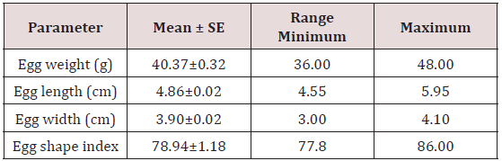
Table 1 shows that the French broiler guinea fowl egg weight ranged from 36 g to 48 g with an average egg weight of 40.37±0.32 g, egg length ranged from 4.55 cm to 5.95 cm with average egg length of 4.86±0.32 cm, egg width ranged from 3.00 cm to 4.10 cm with an average egg width of 3.90±0.02 cm and egg shell index of the French broiler guinea fowls was 78.94±1.18 which ranged from 7.78 to 86.00.

Table 1: Mean Egg Weight and Egg Linear Measurement of the French Broiler Guinea Fowl.

Lupinepublishers-openaccess-Biostatistics-Biometrics-journal

Correlation Between Egg Weight and Egg Linear Measurements of The French Broiler Guinea Fowl

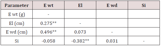
The correlation between egg weight and egg linear measurements is presented in Table 2 Egg weight has a significant (P˂0.01) positive correlation with egg length and egg width, a negative correlation with egg shell index. Egg length has a significant (P˂0.01) positive correlation with egg width, negative correlation with egg shell index. Egg width has significant (P˂0.01) positive correlation with egg weight, positive correlation with egg length and egg shell index. Egg shell index was negatively correlated with egg width, significantly (P˂0.01) negative correlated with egg length and a positive correlation with egg width.

Table 2: Correlation between Egg Weight and Egg Linear Measurement of the French Broiler Guinea Fowl.

Lupinepublishers-openaccess-Biostatistics-Biometrics-journal

Discussion

Mean Egg Weight and Egg Linear Measurement of The French Broiler Guinea Fowl

Variations in egg weight, egg length and egg width observed in this study have also been reported by different researchers [13] observed variations on egg weight and egg length of French broiler and domestic polish guinea fowls raised in the temperate region. [14] reported variations in egg weight, egg length and egg width of Fulani ecotype chicken; [15] also reported variations in egg length, egg width and egg diameter in Fulani and Tiv local chicken ecotype. These variations may be due to the inherent differences between the genetic influence of dams, sires and environmental dissimilarities. Egg size is usually related with body weight of laying hens [16]. In this study, the egg weight of the French broiler guinea fowl strain ranged from 36 g to 48 g while the mean weight was 40.37±0.32 g. The value was lower than the mean weight (55.3 g) for French broiler guinea fowl and similar (40.7g) for domestic polish guinea fowl raised in the temperate region reported by [13,16] reported lower mean values of 37.67±0.2 g and 37.91±0.39 g for pearl and black strains of guinea fowls respectively. However, [17] reported a similar range of between 38 g to 45 g for indigenous guinea fowl in Nigeria [2,18,19]. Also reported similar values to the value reported in this research. The differences observed in this study may be attributed to the different breeds and the different plane of nutrition in the population; also, differences in environmental factors such as uncontrolled mating of the French broiler guinea fowl with the indigenous guinea fowl on free range which must have led to the loss in vigor of the French broiler guinea fowl.

Mean egg length value 4.86±0.02 cm was lower than the value (52.3±0.06 cm) reported by [20]. Mean egg width value (3.90±0.02 cm) was lower than the value (4.49±0.03 cm) reported by [20]. The value for egg shape index reported in this study (78.94±1.18) was close to the value reported by Dudusola [21] for guinea fowl in Nigeria. Nowaczewsky [13] reported lower values of 73.7 cm and 74.4 cm for French broiler guinea fowl and polish domestic strains guinea fowl which did not differ significantly. The differences observed may be due to the differences in breeds, nutrition and management practices. The value for egg shape index observed in this study suggests that eggs are less prone to breakage and can make good for hatchability.

Correlation Between Egg Weight and Egg Linear Measurements

The correlation between egg weight and, egg length and egg width were moderately positive and significant (P<0.01). This implies that as egg weight increases, egg length and egg width also increase. The positive correlations observed in this study between egg weight and, egg length and egg width agree with the results of [22,23]. The relationship between egg length and egg width was low and positive. There was an inverse association between egg length and egg shape index. The reason for this relationship is the fact that egg length is the denominating factor in estimating shape index according to Panda [24,25]. This report agrees with reports of Cloprakan [26]. Egg width showed positive correlation with egg shape index. This is because egg shape index is directly related to egg width. The reason could be as a result of the denser part of the yolk occupying the width area which translates to heavier weight of the egg. This result is similar to results by [27-30] who reported positive correlation between egg weight and egg length.

Conclusion

Egg weight had positive correlation with egg weight and length. Genetic improvement of egg weight can be achieved by selection for egg length and width.

Recommendation

Genetic improvement program for egg weight in the broiler guinea fowl populations in Nigeria can be achieved by selection for egg width and length.

Read More About Current Trends on Biostatistics & Biometrics (CTBB) Please Click on Below Link: https://lupine-publishers-biostatistics.blogspot.com/

Tuesday, 25 May 2021

Lupine Publishers| Orthogonal Arrays and Row-Column and Block Designs for CDC Systems

 Lupine Publishers| Current Trends on Biostatistics & Biometrics (CTBB)


Abstract

In this article, block and row-column designs for genetic crosses such as Complete diallel cross system using orthogonal arrays (p2, r, p, 2), where p is prime or a power of prime and semi balanced arrays (p(p-1)/2, p, p, 2), where p is a prime or power of an odd prime, are derived. The block designs and row-column designs for Griffing’s methods A and B are found to be A-optimal and the block designs for Griffing’s methods C and D are found to be universally optimal in the sense of Kiefer. The derived block and rowcolumn designs for method A and C are new and consume minimum experimental units. According to Gupta block designs for Griffing’s methods A,B,C and D are orthogonally blocked designs. AMS classification: 62K05.

Keywords: Orthogonal Array; Semi-balanced Array; Complete diallel Cross; Row-Column Design; Optimality

Introduction

Orthogonal arrays of strength d were introduced and applied in the construction of confounded symmetrical and asymmetrical factorial designs, multifactorial designs (fractional replication) and so on Rao [1-4] Orthogonal arrays of strength 2 were found useful in the construction of other combinatorial arrangements. Bose, Shrikhande and Parker [5] used it in the disproof of Euler’s conjecture. Ray-Chaudhari and Wilson [6-7] used orthogonal arrays of strength 2 to generate resolvable balanced incomplete block designs. Rao [8] gave method of construction of semi-balanced array of strength 2. These arrays have been used in the construction of resolvable balanced incomplete block design. A complete diallel crossing system is one in which a set of p inbred lines, where p is a prime or power of a prime, is chosen and crosses are made among these lines. This procedure gives rise to a maximum of v =p2 combination. Griffing [9] gave four experimental methods:

parental line combinations, one set of F1’s hybrid and reciprocal F1’s hybrid is included (all v = p2 combination)

parents and one set of F1’s hybrid is included but reciprocal F1’s hybrid is not (v = 1/2 p(p+1) combination)

one set of F1’s hybrid and reciprocal are included but not the parents (v =p(p-1) combination) and

one set of F1’s hybrid but neither parents nor reciprocals F1’s hybrid is included (v = 1/2p(p-1). The problem of generating optimal mating designs for CDC method D has been investigated by several authors Singh, Gupta, and Parsad [10].

For CDC method A, B and C models of Griffing [9] involves the general combining ability (g ca) and specific combining ability (sca) effects of lines. Let nc denote the total number of crosses involved in CDC method A, B and C and it is desired to compare the average effects or g ca effects of lines. Generally, the experiments of these methods are conducted using either a completely randomized design (CRD) or a randomized complete block (RCB) design involving nc crosses as treatments. The number of crosses in such mating design increases rapidly with an increase in the number of lines p. Thus, if p is large adoption of CRD or an RCB design is not appropriate unless the experimental units are extremely homogeneous. It is for this reason that the use of incomplete block design as environment design is needed for CDC method A, B and C. Agarwal and Das [11] used n-ary block designs in the evaluation of balanced incomplete block designs for all the four Griffing’s [9] complete diallel cross (CDC) systems. Optimal block designs for CDC method a and b and variance balanced designs for CDC method c have been constructed by Sharma and Fanta [12,13] but their designs consume more experimental units. This call designs for CDC methods A, B and C which consume less experimental units in comparison to their designs and at the same time are A-optimal or optimal. We restrict here to the estimation of general combining ability (gca) effects only. For analysis of these designs [12-14].

I in the present paper, we are deriving block and row-column designs for complete diallel cross (CDC) system i.e. methods A, B, C and d through orthogonal arrays and semi balanced arrays. Block designs and row-column designs obtained for methods a consume minimum experimental units and are A-optimal. Block designs obtained for method C are optimal in the sense of Kiefer [15] and consume minimum experimental units but row-column designs are neither A-optimal nor optimal. Conversely block designs and row-column designs obtained for methods B are A-optimal. Block designs obtained for method D are optimal in the sense of Kiefer [15] but row-column designs are neither A-optimal nor optimal. The rest of this article is organized as follows: in section B and C we have discussed universal optimality of designs for 1-way and 2-way settings. In section 4 and 5, we give some definitions of orthogonal array, semi balanced arrays and orthogonally blocked design and relation of orthogonal; array with designs for CDC system and optimality with examples and theorems. In section 6 we give relation of semi-balanced array to CDC system along with theorem and for example.

Model and Estimation in 1-Way Heterogeneity Setting

According to Sharma and Tadesse let d be a block design for a CDC systems experiment involving p inbred lines, b blocks each of size k. This means that there are k crosses in each of the blocks of d. Further, let rdt and sdi denote the number of replications of cross t and the number of replications of the line i in different crosses, respectively, in d [ t = 1,2, …, nc; i = 1, 2, …, p]. It is not hard to see that,
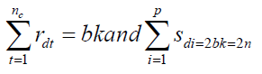
Lupinepublishers-openaccess-Biostatistics-Biometrics-journal

nc = number of crosses and n = bk, the total number of observations. For estimating general combining ability (gca) effects of lines, we took the following linear model for the observations obtained from block design d.

Lupinepublishers-openaccess-Biostatistics-Biometrics-journal

where y is an n×1 vector of observations, 1n is the n×1 vector of ones, △1 is the n × p design matrix for lines and △2 is an n × b design matrix for blocks, that is, the (h,λ)th element of △1 ( respectively, of △1) is 1 if the hth observation pertains to the lth line (respectively, of block) and ois zero otherwise. μ is a general mean, g is a p × 1 vector of line parameters, Β is a b × 1 vector of block parameters and e is an n × 1 vector of residuals. It is assumed that the vector of block parameter, Β is fixed and e is normally distributed with


Lupinepublishers-openaccess-Biostatistics-Biometrics-journal

where I is the identity matrix of conformable order. Using least squares estimation theory with usual restriction Lupinepublishers-openaccess-Biostatistics-Biometrics-journal, we shall have the following reduced normal equations for the analysis of proposed design d, for estimating the general combining ability (gca) effects of lines under model (2.1).

Lupinepublishers-openaccess-Biostatistics-Biometrics-journal

In the above expressions, Gd =△1 △′1 = (gdii´), gdii = sdi and for i ≠i´, gdii´ is the number of crosses in d in which the linesi and i´ appear together. Nd= △1△′2 = (ndij), ndij is the number of times the line i occurs in block j of d and Kd = △2△′2 is the diagonal matrix of block sizes. T = △′1 y and B = △′2 y are the vectors of lines totals and block totals of order p × 1 and b × 1, respectively for design d. A design d will be called connected if and only if rank (Cd) = p -1, or equivalently, if and only if all elementary comparison among general combining ability (gca) effects are estimable using d. We denote by D (p, b, k), the class of all such connected block design {d} with p lines, b blocks each of size k. In section 3, we will discuss Kiefer’s [15] criterion of the universal optimality of D (p, b, k).

Lupinepublishers-openaccess-Biostatistics-Biometrics-journal

Where y is an n × 1 vector of observed responses, μ is the general mean, g, Β and ã are column vectors of p general combining ability (gca) parameters, k row effects and b column effects, respectively, △1(n× p), △'2(n× k), △'3(n×b) are the corresponding design matrices, respectively and e denotes the vector of independent random errors having mean 0 and covariance matrix σ2In.LetNd1 = △1 △'2 be the p × k incidence matrix of lines vs rows and Nd2 = △1 △'3 be the p × b incidence matrix of treatments vs columns and △1△'3= 1k1b.Let rdl denote the number of times the lth cross appears in the design d, λ = 1, 2, . . . , nc and similarly sdi denote the number of times the ith line occurs in design d, i = 1, . . . p. Under (3.1), it can be shown that the reduced normal equations for estimating the gca effects of lines with usual restriction Lupinepublishers-openaccess-Biostatistics-Biometrics-journal, after eliminating the effect of rows and columns, in block design d are
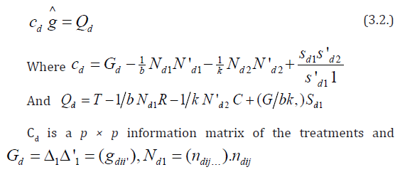
Lupinepublishers-openaccess-Biostatistics-Biometrics-journal

is the number of times line i occurs in row j of d, Nd2= (ndi.t),

ni.t is the number of times the cross i occurs in column t,

sd1 is the replication vector of lines in design d,

Q is a p × 1 vector of adjusted treatments (crosses) total,

T is a p × 1 vector of treatment (line) totals,

R is a k × 1 vector of rows totals,

C is a b ×1 vector of columns totals, respectively, in design d,

G is a grand total of all observations in design d,

Now we state the following theorem of Parsad et al. [16] without proof.

Theorem: Let d* ∈ D1 (p, b, k) be a row - column design and d* ∈ D (p, b, k) be a block design for diallel crosses satisfying

(i) Trace (Cd*) = k-1b {2 k (k-1-2x) + p x (x+1)

(ii) (Cd*) = (p-1)-1k--1 b {2 k (k -1-2x) + p x (x+1)} (Ip - p-1 1p 1′p) is completely symmetric.

Where x = [2k/p], where [z]is the largest positive integer not exceeding z, Ip is an identity matrix of order p and 1p1′p is a p × p matrix of all ones. Then according to Kiefer [15], d*ɛ D1 (p, b, k) or d*∈ D (p, b, k) is universally optimal and in particular minimizes the average variance of the best linear unbiased estimator of all elementary contrasts among the gca effects. Furthermore, using d*ɛ D1 (p, b, k) or d*∈ D (p, b, k) all elementary contrasts among gca effects are estimated with variance.

Lupinepublishers-openaccess-Biostatistics-Biometrics-journal

Some Definitions

Definition 4.1: According to Bose and Bush [17], an r × N matrix A, with entries from a set ∑ of p ≥ 2 elements is called an orthogonal array of strength d, size N, r constraints and p levels if d × N sub matrix of A contains all possible × 1 column vectors with the same frequency λ. The array may be denoted by (N, r, p, d). The number λ may be called the index of the array. Clearly N = λ pd.

Definition 4.2: According to Rao [8], a (N, r, p) array is said to be a semi-balanced array of strength d if for any selection of d rows α1, α2, . . . , αd, we denote d rows by n(i1, i2, . . ., id).

(i) n (i1, i2, . . ., id) = 0 if any two ij are equal.

Lupinepublishers-openaccess-Biostatistics-Biometrics-journal

Where s represents summation over all permutation of distinct elements i1 , i2, . . ., id.

Definition 4.3: According to Gupta et al. [18], a diallel cross design to be orthogonally blocked if each line occurs in every block r/b time, where r is the constant replication number of the lines and b is the number of blocks in the design.

Relation between Orthogonal Array (p2, p+1, p, 2) and Designs for CDC System

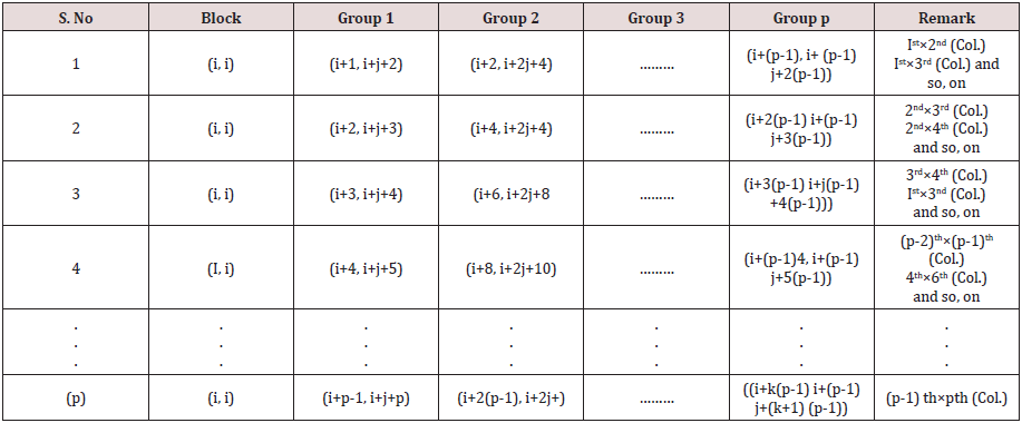
Consider an orthogonal array (p2, p+1, p, 2), where p is a prime or power of a prime. If we divide this array into p groups where each group contains p × (p+1) elements and identify the elements of each group as p lines of a diallel cross experiments. Now we perform crosses in any two columns of (p+1) constraints in first group and perform crosses among the lines appearing in the corresponding columns in (p-1) groups, we get p initial columns blocks as given below, which can be developed cyclically mod(p) to get design d1 for diallel cross experiment Griffing’ s method A with p2 distinct crosses of p parental lines consisting of p self, 1/2 p (p-1) number of F1 crosses, and the same number of reciprocal F1’s with parameter v = p2, b = p, k =p , r =1. By this procedure we obtain p(p+1)/2 designs for diallel cross experiment Griffing’s method A (Table1). Note: All column blocks will be developed cyclically mod (p).

Table 1:
Lupinepublishers-openaccess-Biostatistics-Biometrics-journal

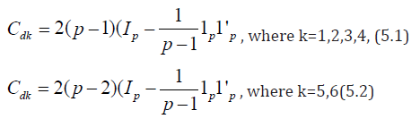
Now considering in d1 , the cross of the type (i, j) = (j, i), i, j = 1,2, . . . p, we may obtain design d2 for Griffing’s method B with parameters v = p(p+1)/2, b =p, k =p, r1 =1,for cross of the type (i, i) and r2 =2, for cross of the type (i, j), where i, j = 1, 2, . . ., p, respectively. Considering rows as row blocks in block designs d1 and d2 we may also obtain row-column designs d3 and d4 for Griffing’s methods A and B with parameters v = p2, b = p, k =p, r =1 and v = p(p+1)/2, b =p, k =p, r1 =1,for cross of the type (i,i) and r2 =2, for cross of the type (i, j), where i, j = 1, 2, . . ., p, respectively. If we ignore the crosses of the type (i, i) in d1, where i = 1, 2, . . . p, we may obtain the block design d5 for Griffing’s method C with parameters v = p (p-1), b =p, k =p and r =1. Considering the crosses of the type (i, j) = (j, i) in d5 we may also derive design d6 for Griffing’s method D with parameters v = p (p-1)/2, b =p, k =p and r =1, where i < j = 1, 2,. . ., p. Considering rows as row blocks in block designs d5 and d6, we may also derive row-column designs d7 and d8 for Griffing’s methods C and D with parameters v = p (p-1), b =p, k =p , r =1 and v = p(p-1)/2, b =p, k =p and r =1, respectively, The designs d7 and d8 are neither optimal nor A-optimal. It is not hard to see that block and row-column designs obtained for Griffing’s methods A and C consume minimum experimental units and in theses designs every cross is replicated only once and each line occurs in every block r/b time, where r is the constant replication number of line and b is the number of blocks in the design. In block designs for Griffing’s methods B and D each line also occurs in every block r/b time. Hence according to Gupta et al. [18] these designs are orthogonally blocked. In an orthogonal design no loss of efficiency on the comparisons of interest is incurred due to blocking. A block design for which N = θ 1p 1′b is orthogonal for estimating the contrasts among gca parameters, where N denotes the line versus block incidence matrix and θ is some constant. For designs dk ∈ D (p, b, k), where k = 1, 2, 5, and 6 and designs dk ∈ D1 (p, b, k), where k = 3, 4, we have ndkij = 2, for k =1, 2,. . ., 8; i =1, 2, . . .p, j = 1, 2,. . ., p and their information matrices Cdk are as given below.
Lupinepublishers-openaccess-Biostatistics-Biometrics-journal

Where Ip is an identity matrix of order p and 1p is a unit column vector of ones. Clearly Cdk given by (5.1) is completely symmetric and Trace ( Cdk ) = 2 (p-1)2 which is not equal to the upper bound given in (5.3).

Lupinepublishers-openaccess-Biostatistics-Biometrics-journal

Hence the designs d1, d2, d3, and d4 are not optimal. The information matrix Cdk given by (5.2) is completely symmetric and Trace ( Cdk ) = 2 (p-1) (p-2) which is equal to the trace given in (5.3). Hence the designs d5 and d6 are optimal in the sense of Kiefer [15] and in particular minimizes the average variance of the best linear unbiased estimator of all elementary contrasts among the gca effects. To prove that the designs d1, d2, d3, and d4 are A- optimal, we consider the following criteria. A design d* ∈ D (p, b, k) is said to be A-optimal in D (p, b, k) if and only if Trace ((Vd*)≤Trace(Vd))

Here d* denotes designs d1, d2, d3, and d4 and d denotes designs d5 and d6. The Trace (Vd*) is equal to 1/2 and Trace (Vd*) is which is greater than 1/2.Hence designs d1, d2, d3, and d4 are an A-optimal.

Remark: The variances of the best linear unbiased estimators of elementary contrasts among gca effects are equal in A-optimal designs and also in optimal designs. It means that all the designs are variance balanced, this fact is particularly attractive to the experimenter, as it enables one to carry out the analysis of the experiment in an extremely simple manner.

Now we state the following theorems.

Theorem: The existence of an Orthogonal Array (p2, p+1, p, 2) implies the

existence of Lupinepublishers-openaccess-Biostatistics-Biometrics-journal different layouts A- optimal incomplete block designs with parameters v = p2, b = p, k =p, r =1.

(ii) existence Lupinepublishers-openaccess-Biostatistics-Biometrics-journal different layouts A- optimal incomplete designs for Griffing’s method B with parameters v = p (p+1)/2, b =p, k =p, r1 =1, for cross of the type (i, i) and r2 =2, for cross of the type (i, j), where i, j = 1, 2, . . ., p, respectively.

(iii) existence of p(p-1)/2 row-column designs for Griffing’s [9] methods A and B with parameter v = p2, b = p, k =p , r =1 and v = p (p+1)/2, b =p, k =p , r1 =1,for cross of the type (i, i) and r2 =2, for cross of the type (i, j), where i, j = 1, 2, . . ., p, respectively.

Theorem:- The existence of an Orthogonal Array (p2, p+1, p, 2) implies the existence of Lupinepublishers-openaccess-Biostatistics-Biometrics-journal different layouts optimal incomplete block designs for Griffings [9] methods C and D with parameters v = p(p-1), b =p, k =p , r =1 and v = p(p-1)/2, b =p, k =p and r =1, respectively.

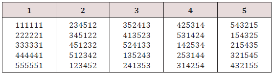
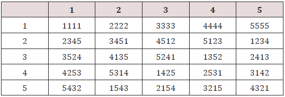
Example: Following Rao [19] we construct an orthogonal array (25,6,5,2) of rp =5, the 4 orthogonal Latin squares with bordered elements are (Table 2). This arrangement may be expressed in five groups as given below Table 3. The above arrangement is an orthogonal array (25, 6, 5, 2). From the above array we can derive the designs for the four experimental methods described by Griffing [9]. The procedure is explained below.

Table 2:
Lupinepublishers-openaccess-Biostatistics-Biometrics-journal

Table 3:

Lupinepublishers-openaccess-Biostatistics-Biometrics-journal

For Griffing methods A and B, we can take any two columns from first group and corresponding columns from other groups i.e. 2, 3, 4, and 5 and arrange them in columns and then we obtain design for methods A and B. Thus, we may obtain 14 different layouts designs for each method A and method B. We may also obtain 10 different layouts row-column designs for each of these methods A and B.

Remark: - Block and row column designs for methods A and B containing crosses with last column of group 1 are neither A-optimal nor optimal.

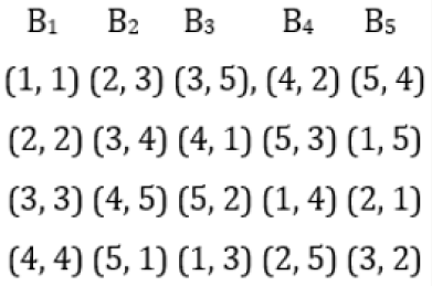
Example: Suppose we take the first two columns from first group and corresponding columns from other groups i.e. 2, 3, 4, and 5. Elements in brackets are considered cross between lines and then we obtain the following design for Griffing’s experimental methods A and B with parameters v = 25, b = 5, k =5, and r =1 and v = 15, b = 5, k =5, and r =1, respectively, with the condition that the cross (i, j) = (j, i) for method (2), where i < j = 1, 2, . . ., 5.

Figure 1 In the above design, considering rows as row blocks, we may we may obtain row-column designs for Griffing’s methods A and B respectively. From the above design we may also derive designs for methods C and D by ignoring the first column and considering (i, j) ≠ (j, i), in other columns, where i, j = 1, 2, 3, 4, and 5, with parameters v = 20, b = 5, k =5, and r =1. In Griffing’s method C design considering (i, j) = ( j, i) , where i< j = 1,2, 3, 4, and 5, we obtain a design for CDC method D with parameters v = 10, b = 5, k =5,and r =2, Thus, from the above array we may obtain 10 different layouts of designs for method C and 10 different layouts of designs for method D.

Figure 1: Design for Griffing’s Method A and B.
Lupinepublishers-openaccess-Biostatistics-Biometrics-journal

Relation between Semi-Balanced Array (p(p-1)/2, p, p, 2) and Designs for CDC System

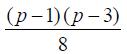
Consider a semi-balanced (p(p-1)/2, p, p, 2), where p is an odd prime or power of odd prime. There are (p-1)/2 total sets in a semi-balanced (p(p-1)/2, p, p, 2). If we identify the elements of semibalanced array as lines of a diallel cross experiment and perform crosses in any two sets among the corresponding lines appearing in the same two sets, we get a mating design for diallel cross experiment involving p lines with v =p2crosses, each replicated once. The mating design can be converted into block design for diallel cross experiment Griffing’s methods A with parameter v = p2, b = p, k =p and r =1, considering rows as blocks. In the above design considering the cross (i, j) = (j, i) where i < j = 0, 1, 2, . . ., p, we obtain design for Griffing’s method B with parameters v = p(p+1)/2, b =p, k =p , r1 =1,for cross of the type (i, i) and r2 =2, for cross of the type (i, j), where i, j = 1, 2, . . ., p, respectively.. From block designs obtained for methods A and B we may also obtain row-column designs for Griffing’s methods A and B by considering columns as row blocks with parameters v = p2, b = p, k =p and r =1 and v = p(p+1)/2, b =p, k =p , r1 =1,for cross of the type (i,i) and r2 =2, for cross of the type (i, j), where i, j = 1, 2, . . ., p, respectively. From the above mating design deleting the first row and considering (i, j) ≠ ( j, i), where i < j = 0, 1, . . ., p we can also derive designs for methods C, with parameters with parameters v = p (p-1), b =p, k =p , r =1. Considering (i, j) = (j, i), where i, j = 0, 1, . . ., p, we obtain design for Griffing’s method D with parameters v = p(p-1)/2, b =p, k =p and r =2. Thus, using above techniques, we may obtain Lupinepublishers-openaccess-Biostatistics-Biometrics-journal different layouts designs for Griffing’s methods A, B, C and D. The information matrices of block designs and row-column designs for methods A and B are same as given in (1). So, block designs and row-column designs for methods A and B are A- optimal. Similarly, the information matrices of designs for methods C and D are the same as given in (1), so designs for methods C and D are universally optimal in the sense of Kiefer [15] and in particular minimizes the average variance of the best linear unbiased estimator of all elementary contrasts among the gca effects. These designs are orthogonally blocked. Now we state the following theorems.
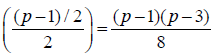
Theorem 1: The existence of semi -balanced array (p(p-1), p, p, 2) implies the existence of different layouts of Lupinepublishers-openaccess-Biostatistics-Biometrics-journal A- optimal incomplete block designs and row-column designs for Griffing’s [9] methods A and B with parameters v = p2, b = p, k =p and r =1 and v = p(p+1)/2, b =p, k =p and r =1,respectively, where we consider the cross (i, j) = (j, i) for method B, where i < j = 0, 1, 2, . . ., p.
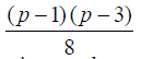
Theorem 2: The existence of Semi -Balanced Array (p (p-1), p, p, 2) implies the existence of Lupinepublishers-openaccess-Biostatistics-Biometrics-journal different lay outs of optimal incomplete block designs v = p(p-1), b =p, k =p and r =1 and v = p(p-1)/2, b=p, k=p and r=2, respectively, for Griffing’s [9] methods C and D.
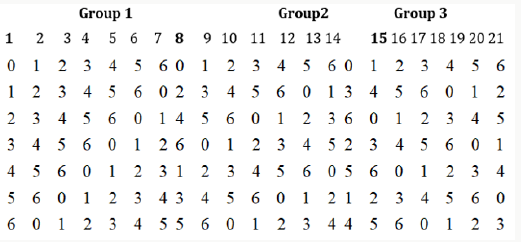
Example. If p =7, the residue classes 0, 1, . . . , 6 (mod7) form a field . We write the 7 elements of GF (7) as 0, ±1, ±2, ±3 and hence the key sets are, using the formula (7.1), where

(0, 1, 2, 3, 4, 5, 6), (0, 2, 4, 6, 1, 3, 5), and (0, 3, 6, 2, 5, 1, 4) (8.1)

second and third vectors are obtained from the first on multiplying by 2 and 3, respectively. Writing (8.1) vertically (shown in bold numbers) and generating the other columns by the addition of elements GF (7) as indicated in (7.3). We obtain 21 columns as shown below which is divided into three groups (Figure2).

Figure 2:
Lupinepublishers-openaccess-Biostatistics-Biometrics-journal

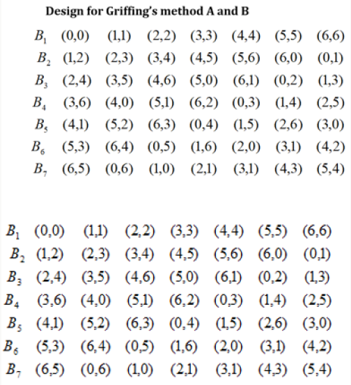
From the semi balanced array given above, we may obtain designs for Griffing’s four experimental methods by superimposing group 2 over group 1 or group 3 over group1 or group 3 over group 2. We superimpose group 2 over group 1 and obtain following design for Griffing’s methods A and B with parameters v =49, b = 7, k =7, and r1 =1 and v = 28, b = 7, k =7, and r =1, with the condition that the cross (i, j) = (j, i), where i < j = 0, 1, 2, . . ., 6 (Figure 3).

From the above design we can derive designs for methods C, and D

Figure 3:
Lupinepublishers-openaccess-Biostatistics-Biometrics-journal

(i) By ignoring the first row and considering (i, j) ≠ (j, i) in other rows, where i < j = 0, 1, . . ., 6, for method C and

(ii) similarly ignoring first row and taking other rows and also considering (i, j) = (j, i) in other rows, where i, j = 0, 1, . . ., 6, thus we may obtain Lupinepublishers-openaccess-Biostatistics-Biometrics-journal different layouts of designs for method C and D.

Conclusion

In the present article we have given block and row-column designs for Griffing’s CDC system i.e for all methods A, B, C, and D by using orthogonal array (p2, p+1, p, 2) and semi -balanced array (p(p-1), p, p, 2). Block and row-column designs for methods A and block designs for method C consume minimum experimental units and are A-optimal and optimal, respectively. These designs are.


Read More About  Current Trends on Biostatistics & Biometrics (CTBB) Click on Below Link:

https://lupine-publishers-biostatistics.blogspot.com/