In quantum optics, the Heisenberg picture, in which the
optical fields can be treated as conjugate positions and momenta of
quantized harmonic oscillators, as it is easy to substitute
optical fields in classical electromagnetic problems with noncommutative
operators and obtain the Heisenberg equations of motion. Once
the operator equations are solved, it is possible obtain various
quantum properties of the optical fields via noncommutative
algebra. The Heisenberg picture is often not without shortcomings. Its
difficulties have led to a growing appreciation of the
Schrödinger picture, where the photons are treated as an ensemble of
bosons
and the evolution of the many-photon probability can be used.
This is more intuitive approach that has led to great success in the
quantum theory of solitons. Instead of solving the formidable
nonlinear operator equations, we can obtain analytic solutions from
the linear boson equations in plasmatic the Schrödinger picture
which lead to the theory of Plasmatic Moving Frames.
Keywords: The Heisenberg Picture; The Optical Fields; The Plasma in Physics; Plasma in Medicine; The Many Photon Probability;
Solitons, The Schrödinger Picture; Nonlinear Operator Equations; Plasmatic Moving Frame
Introduction
Plasma
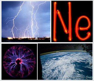
(Figure 1) Plasma (from Ancient Greek πλάσμα, meaning
‘moldable substance [1]) is one of the four fundamental states of
matter, and was first described by chemist Irving Langmuir [2] in
the 1920s [3]. Plasma can be artificially generated by heating or
subjecting a neutral gas to a strong electromagnetic field to the
point where an ionized gaseous substance becomes increasingly
electrically conductive, and long-range electromagnetic fields
dominate the behaviour of the matter [4]. Plasma and ionized
gases have properties and display behaviors unlike those of the
other states, and the transition between them is mostly a matter
of nomenclature [2] and subject to interpretation [5]. Based on
the surrounding environmental temperature and density, partially
ionized or fully ionized forms of plasma may be produced. Neon
signs and lightning are examples of partially ionized plasma [6].
The Earth’s ionosphere is a plasma and the magnetosphere contains
plasma in the Earth’s surrounding space environment. The interior
of the Sun is an example of fully ionized plasma, [7] along with the
solar corona [8] and stars [9]. Positive charges in ions are achieved
by stripping away electrons orbiting the atomic nuclei, where the
total number of electrons removed is related to either increasing
temperature or the local density of other ionized matter. This also
can be accompanied by the dissociation of molecular bonds, [10]
though this process is distinctly different from chemical processes
of ion interactions in liquids or the behaviour of shared ions in
metals. The response of plasma to electromagnetic fields is used
in many modern technological devices, such as plasma televisions
or plasma etching [11]. Plasma may be the most abundant form of
ordinary matter in the universe, [12] although this hypothesis is
currently tentative based on the existence and unknown properties
of dark matter. Plasma is mostly associated with stars, extending
to the rarefied intracluster medium and possibly the intergalactic
regions [13].
Definition
Plasma is a state of matter in which an ionized gaseous
substance becomes highly electrically conductive to the point
that
long-range electric and magnetic fields dominate the behaviour
of
the matter. The plasma state can be contrasted with the other
states:
solid, liquid, and gas. Plasma is an electrically neutral
medium of
unbound positive and negative particles (i.e. the overall
charge of a plasma is roughly zero). Although these particles are
unbound,
they are not “free” in the sense of not experiencing forces.
Moving
charged particles generate an electric current within a
magnetic
field, and any movement of a charged plasma particle affects
and
is affected by the fields created by the other charges. In
turn this
governs collective behaviour with many degrees of variation
[10].
Figure 1: Top: Lightning and neon lights are commonplace generators of plasma. Bottom left: A plasma globe, illustrating some
of the more complex plasma.
Mathematical Descriptions
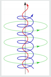
(Figure 2) The complex self-constricting magnetic field lines and
current paths in a field aligned Birkeland current that can develop
in a plasma. To completely describe the state of a plasma, all of the
particle locations and velocities that describe the electromagnetic
field in the plasma region would need to be written down. However,
it is generally not practical or necessary to keep track of all the
particles in a plasma. Therefore, plasma physicists commonly use
less detailed descriptions, of which there are two main types:
Figure 2.
a) Fluid Model
Fluid models describe plasmas in terms of smoothed quantities,
like density and averaged velocity around each position (see Plasma
parameters). One simple fluid model, magnetohydrodynamics,
treats the plasma as a single fluid governed by a combination of
Maxwell’s equations and the Navier–Stokes equations. A more
general description is the two-fluid plasma picture, where the ions
and electrons are described separately. Fluid models are often
accurate when collisional is sufficiently high to keep the plasma
velocity distribution close to a Maxwell–Boltzmann distribution.
Because fluid models usually describe the plasma in terms of a
single flow at a certain temperature at each spatial location, they
can neither capture velocity space structures like beams or double
layers, nor resolve wave-particle effects.
b) Kinetic Model
Kinetic models describe the particle velocity distribution
function at each point in the plasma and therefore do not need
to
assume a Maxwell–Boltzmann distribution. A kinetic description
is
often necessary for collision less plasmas. There are two
common
approaches to kinetic description of a plasma. One is based on
representing the smoothed distribution function on a grid in
velocity and position. The other, known as the
particle-in-cell (PIC)
technique, includes kinetic information by following the
trajectories
of a large number of individual particles. Kinetic models are
generally more computationally intensive than fluid models.
The
Vlasov equation may be used to describe the dynamics of a
system
of charged particles interacting with an electromagnetic
field. In magnetized plasmas, a gyrokinetic approach can substantially
reduce the computational expense of a fully kinetic simulation.
c) The spatiotemporal entanglement evolution in free
space
The many-boson interpretation may be applied to study of
entangled photons as well, where the two-photon probability is
used to obey the Wolf equations by Saleh, Teich, and Sergijenko
(STS). Instead of treating the entanglement properties of the
photons, and the optical propagation as two separate problems,
with the STS equations, we can use now a single quantity – namely,
the two-photon amplitude – to keep track of the spatiotemporal
entanglement evolution in free space. This is analogous to the
Wolf equations, which reformulate the laws of optics in terms of
coherence propagation. We utilize the STS treatment of the two
photons in study of various temporal effects. The Schrödinger
picture would offer a more accessible interpretation of temporal
entanglement propagation for studies of two-photon systems.
For example, a four-wave mixing in a coherently prepared atomic
gas, thus extending the STS model for use in many more topics in
quantum optics in order to demonstrate the use and intuitiveness
of the Schrödinger picture. Based on this formalism, we propose
the concept of quantum plasmatic temporal imaging, which uses
dispersive elements and temporal phase modulators to manipulate
the temporal entanglement properties of two photons. It is possible
to convert positive-time correlation to negative-time correlation, or
vice versa, using a plasmatic temporal imaging system.
This conversion technique could be immensely useful for
applications that require negative-time correlation, such as
quantum-enhanced clock synchronization. Generating of
negativetime correlation directly has some shortcomings compared with
the conventional tried-and-true schemes that generate
positivetime correlation. This technique could allow more flexibility in
choosing two-photon sources for quantum optics applications.
We can consider two photons in two optical modes, such as two
polarization, two propagation directions, or two waveguide
modes.
The two-photon wave function is

Where the constants C s are overall amplitudes of the
quantum
states, is the quantum state in which one photon is in each
mode,
is the state in which both photons are in mode 1 and is the
state in
which both photons are in mode 2. The positive-frequency
forwardpropagating component of the electric field in each mode is given
by

Where  is the complex, frequency-dependent refractive index
in mode
is the complex, frequency-dependent refractive index
in mode  , is the real part of
  , S is an area of quantization in the
x-y plane, and
, S is an area of quantization in the
x-y plane, and  is the photon annihilation operator, related to the
corresponding creator operator via the equal-space commutator
is the photon annihilation operator, related to the
corresponding creator operator via the equal-space commutator

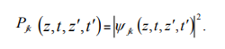
The physical significance of each amplitude  is that
its magnitude squared gives the probability density
is that
its magnitude squared gives the probability density  of
coincidentally measuring one photon in mode j at (z,t) and another
photon in mode k at
of
coincidentally measuring one photon in mode j at (z,t) and another
photon in mode k at  ,
,
Plasmatic temporal entanglement is defined as irreducibility of
into a product of one-photon amplitudes in the form of a(t)b(  ).
This means that the probability of detecting a photon in mode 1 at
time t is correlated to the probability of detecting a photon in mode
2 at
).
This means that the probability of detecting a photon in mode 1 at
time t is correlated to the probability of detecting a photon in mode
2 at  . The most popular ways of generated entangled photons are
spontaneous parametric down-conversion and four-wave mixing,
where wave-mixing geometry and the spatiotemporal profile of the
pump-beam determine the initial
. The most popular ways of generated entangled photons are
spontaneous parametric down-conversion and four-wave mixing,
where wave-mixing geometry and the spatiotemporal profile of the
pump-beam determine the initial  . (17, 18)
The most interesting case is when M=-1 and one of the photons
is time reversed. If the two photons are initially entangled with
positive-time correlation can be written as  , where b is assumed to be much sharper than a. After photon
1 has passed through the plasmatic temporal imaging system M=-1
, where b is assumed to be much sharper than a. After photon
1 has passed through the plasmatic temporal imaging system M=-1 The photons hence become
anticorrelated in time. Since most conventional two-photon sources
generate positive-time correlation, but negative-time correlation is
desirable for many applications, one can use the temporal imaging
system to convert the former to the latter.
The photons hence become
anticorrelated in time. Since most conventional two-photon sources
generate positive-time correlation, but negative-time correlation is
desirable for many applications, one can use the temporal imaging
system to convert the former to the latter.
Besides the above application, one can also convert
negativetime correlation, which can be generated by ultrashort pulses
for
improved efficiency, to positive correlation. Any desired
correlation
can actually be imposed on already entangled photons, by
multiplying the original correlation with a factor of 1/M. As
groupvelocity dispersion and temporal phase modulation play analogous
roles in the time domain to diffraction and lenses, which can
be use
Fourier optics, temporal imaging, and quantum imaging
techniques
to design more complex quantum plasmatic temporal imaging
systems. The quantum destructive interference via a coupler is
determined by the overlap of the two photons amplitude with
its
plasmatic mirror image. The output amplitude is the
destructive
interference between the original amplitude and its replica
but with
the two photons exchanging their positions in time. In
particular, for
a 50%-50% coupler, T=R=1/2, complete destructive interference
is produced if the two photons are temporarily
indistinguishable.
The introduction of variable distinguishability to photons, in
order
to produce varying degrees of destructive interference via a
beam
splitter to measure the two-coherence time, is the basic
principle
of the Hong-Ou-Mandel interferometer. As envisioned by Lukin
and
Imamoglu, the third-order nonlinear effects among two photons
can become significant in a coherently prepared plasmatic
atomic gas. The coupled-mode equations and then become nonlinear,
where is the self-phase modulation coefficient and also
cross-phase
modulation coefficient. The advantage of the Schrödinger
picture is
most evident, whereas in the Heisenberg picture one needs to
solve
nonlinear coupled-mode operator equations, in the Schrödinger
picture, one only needs to solve linear equations, which are
similar
to the configuration-space model applied to the quantum theory
of solitons. The delta function couples the two subspaces, so
entanglement can emerge from unentangled photons. A soliton
formed by two photons in orthogonal polarizations exerting
crossphase modulation on each other. Studies of two photons in the same
mode under the self-phase modulation effect have been
performed
by entanglement, and cross-phase modulation offers the
distinct
possibility of entangling two photons in different modes.
Consider the case in which two polarizations have the same
group-velocity dispersion, so that, and there is one photon in each
polarization. The evolution equation for

Defining time coordinates in a plasmatic moving frame.

we obtain the following equation for  :
:

This equation is a simple linear Schrödinger equation,
describing a two-dimensional “wave function”  in
a moving frame subject to a
in
a moving frame subject to a  potential. To solve for
explicitly, we define new time coordinates
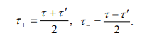
The cross-phase modulation effect only offers confinement of
along the time difference
 axis, but not the mean arrival time
  axis. The only
bound-state solution of is
axis. The only
bound-state solution of is

The delta potential enforces S to take on the value  where
where
 and
and  must have opposite signs.
For the final solution in the plasmatic moving frame of  and
and  is therefore

The two-photon coherence time of a vector soliton is fixed,
but he average arrival time is still subject to dispersive spreading
and becomes increasingly uncertain as they propagate. Hence a
two-photon vector soliton generates temporal entanglement with
positive-time correlation as it propagates. Similar to the idea of
soliton momentum squeezing, one can also abiotically change
along the propagation axis to control independently the two-photon
coherence time. The center frequencies of the photons are shifted
slightly, by an amount of to compensate for their group-velocity
mismatch, so they can copropagating at average group velocity.
This is commonly known as soliton trapping. If the nonlinearity
has a finite bandwidth, the potential becomes a finite-bandwidth
function and multiple bound-state solutions can be obtained via
conventional techniques of solving the linear the Schrödinger
equation.
We have derived the general equations that govern the temporal
evolution of two-photon probability amplitudes in different
coupled optical modes. The formalism inspires the concept of
quantum temporal imaging, which can manipulate the temporal
entanglement of photons via conventional imaging techniques.
The theory also offers an intuitive interpretation of two-photon
entanglement evolution, as demonstrated by the exact solution of
the two-photon vector soliton. To conclude, we expect the proposed
formalism to be useful for many Plasmatic Moving Frames, quantum
signal processing and communication applications.
Plasma Medicine
Plasma sources used in plasma medicine are typically “low
temperature” plasma sources operated at atmospheric pressure.
In this context, low temperature refers to temperatures similar to
room temperature, usually slightly above. There is a strict upper
limit of 50°C when treating tissue to avoid burns. The plasmas are
only partially ionized, with less than 1 ppm of the gas being charged
species, and the rest composed of neutral gas.
a) Dielectric-barrier discharges
Dielectric-barrier discharges are a type of plasma source
that limits the current using a dielectric that covers one or
both
electrodes. A conventional DBD device comprises two planar
electrodes with at least one of them covered with a dielectric
material and the electrodes are separated by a small gap which
is called the discharge gap. DBDs are usually driven by high
AC
voltages with frequencies in the kHz range. In order to use DC
and
50/60 Hz power sources investigators developed the Resistive
Barrier Discharge (RBD) [3]. However, for medical application
of
DBD devices, the human body itself can serve as one of the two
electrodes making it sufficient to devise plasma sources that
consist
of only one electrode covered with a dielectric such as
alumina or
quartz. DBD for medical applications [4] such as for the
inactivation
of bacteria, [5] for treatment of skin diseases and wounds,
tumor
treatment [6] and disinfection of skin surface are currently
under investigation. The treatment usually takes place in the room air.
They are generally powered by several kilovolt biases using
either
AC or pulsed power supplies.
b) Atmospheric Pressure Plasma Jets
Atmospheric pressure plasma jets (APPJs) are a collection
of plasma sources that use a gas flow to deliver the reactive
species generated in the plasma to the tissue or sample. The gas
used is usually helium or argon, sometimes with a small amount
(< 5%) of O2, H2O or N2 mixed in to increase the production of
chemically reactive atoms and molecules. The use of a noble
gas keeps temperatures low and makes it simpler to produce
a stable discharge. The gas flow also serves to generate a region
where room air is in contact with and diffusing into the noble
gas, which is where much of the reactive species are produced
[7]. There is a large variety in jet designs used in experiments
[8]. Many APPJs use a dielectric to limit current, just like in a
DBD, but not all do. Those that use a dielectric to limit current
usually consists of a tube made of quartz or alumina, with a high
voltage electrode wrapped around the outside. There can also be
a grounded electrode wrapped around the outside of the dielectric
tube. Designs that do not use a dielectric to limit the current use a
high voltage pin electrode at the center of the quartz tube. These
devices all generate ionization waves that begin inside the jet and
propagate out to mix with the ambient air. Even though the plasma
may look continuous, it is actually a series of ionization waves or
“plasma bullets”.(8) This ionization wave may or may not treat the
tissue being treated. Direct contact of the plasma with the tissue
or sample can result in dramatically larger amounts of reactive
species, charged species, and photons being delivered to the sample
[9]. One type of design that does not use a dielectric to limit the
current is two planar electrodes with a gas flow running between
them. In this case, the plasma does not exit the jet, and only the
neutral atoms and molecules and photons reach the sample. Most
devices of this type produce thin (mm diameter) plasma jets, larger
surfaces can be treated simultaneously by joining many such jets
or by multielectrode systems. Significantly larger surfaces can be
treated than with an individual jet. Further, the distance between
the device and the skin is to a certain degree variable, as the skin is
not needed as a plasma electrode, significantly simplifying use on
the patient. Low temperature plasma jets have been used in various
biomedical applications ranging from the inactivation of bacteria to
the killing of cancer cells [10].
Applications
Plasma medicine can be subdivided into three main fields:
a) Non-thermal atmospheric-pressure direct plasma for
medical therapy.
b) Plasma-assisted modification of bio-relevant surfaces.
c) Plasma-based bio-decontamination and sterilization.
Non-thermal atmospheric-pressure plasma
One of challenges is the application of non-thermal plasmas
directly on the surface of human body or on internal organs.
Whereas for surface modification and biological decontamination
both low-pressure and atmospheric pressure plasmas can be used,
for direct therapeutic applications only atmospheric pressure
plasma sources are applicable. The high reactivity of plasma is a
result of different plasma components: electromagnetic radiation
(UV/VUV, visible light, IR, high-frequency electromagnetic fields,
etc.) on the one hand and ions, electrons and reactive chemical
species, primarily radicals, on the other. Besides surgical plasma
application like argon plasma coagulation (APC), [11] which is
based on high-intensity lethal plasma effects, first and sporadic
non-thermal therapeutic plasma applications are documented in
literature [12]. However, the basic understanding of mechanisms
of plasma effects on different components of living systems is in
the early beginning. Especially for the field of direct therapeutic
plasma application, a fundamental knowledge of the mechanisms
of plasma interaction with living cells and tissue is essential as a
scientific basis.
Mechanisms
Though many positive results have been seen in the
experiments, it is not clear what the dominant mechanism of action
is for any applications in plasma medicine. The plasma treatment
generates reactive oxygen and nitrogen species, which include free
radicals. These species include O, O3
, OH, H2
O2
, HO2
, NO, ONOOH
and many others. This increase the oxidative stress on cells, which
may explain the selective killing of cancer cells, which are already
oxidatively stressed [13]. Additionally, prokaryotic cells may be
more sensitive to the oxidative stress than eukaryotic cells, allowing
for selective killing of bacteria.
It is known that electric fields can influence cell membranes from
studies on electroporation. Electric fields on the cells being treated
by a plasma jet can be high enough to produce electroporation,
which may directly influence the cell behavior, or may simply allow
more reactive species to enter the cell. Both physical and chemical
properties of plasma are known to induce uptake of nanomaterials
in cells. For example, the uptake of 20 nm gold nanoparticles can
be stimulated in cancer cells using non-lethal doses of cold plasma.
Uptake mechanisms involve both energy dependent endocytosis
and energy independent transport across cell membranes [14]. The
role of the immune system in plasma medicine has recently become
very convincing. It is possible that the reactive species introduced
by a plasma recruit a systemic immune response [15].
Conclusion
For the first time ever, physicists have captured an image of
quantum entanglement. In a paper published in the journal of
Scientific Advances, scientists from the University of
Glasglow
shared the first known image of a Bell entanglement. The photo
depicts two photons interacting and sharing physical states for
a brief instant -- an event that occurs regardless of the
actual
distance between the particles [16]. To capture a picture of
the Bell
entanglement, physicists created a system that shoots off
streams of
entangled photons from a quantum source of light at what they
call
“non-conventional objects.” These objects are displayed on
liquidcrystal materials, which can change the phase of the photons as
they
move through them. A camera capable of detecting photons was
then set to snap a photo when it identified one photon
entangled
with another. According to the researchers, quantum
entanglement
is one of the primary pillars of quantum mechanics. The
concept
is used in practical applications like quantum computing and
cryptography, but no one has ever managed to capture an image
of
it in action. Physicists involved in the project believe that
the image
can help to advance the field of quantum computing and lead to
new types of imaging [16-19]. These results confirm our theory
on
the Plasmatic Moving Frames (PMF).
The Transfiguration
As he was praying, the appearance of Jesus’s face changed,
and
his clothes became as bright as a flash of lightning [20].
While he
was speaking, a cloud appeared and enveloped them, and they
were afraid as they entered the cloud. (35) A voice came from
the
cloud, saying, “This is my Son, whom I have chosen; listen to
him.
LUKE 9: 29-36 These possible transfigurations is part of the
abovementioned new types of imaging, what explanation and proves our
theory of Plasmatic Moving Frames in quantum physics and optics.
Read More Lupine Publishers Otolaryngology Journal Articles:
https://lupine-publishers-otolaryngology.blogspot.com/