Summary
We give a chronological review of the major model selection methods that have been proposed from circa 1960. These model
selection procedures include Residual mean square error (MSE), coefficient of multiple determination (R2), adjusted coefficient of
multiple determination (Adj R2), Estimate of Error Variance (S2), Stepwise methods, Mallow’s Cp,
Akaike information criterion (AIC),
Schwarz criterion (BIC). Some of these methods are applied to a problem
of developing a model for predicting tumors in childhood
using log-linear models. The theoretical review will discuss the problem
of model selection in a general setting. The application will
be applied to log-linear models in particular.
Keywords: MSE; R2; Adj R2; (S2); Stepwise methods; Cp; AIC; BIC
Introduction
Historical Development
The problem of model selection is at the core of progress
in science. Over the decades, scientists have used various
statistical tools to select among alternative models of data.
A common challenge for the scientist is the selection of the
best subset of predictor variables in terms of some specified
criterion. Tobias Meyer (1750) established the two main
methods, namely fitting linear estimation and Bayesian
analysis by fitting models to observation. The 1900 to 1930’s
saw a great development of regression and statistical ideas
but were based on hand calculations. In 1951 Kullback
and Leibler developed a measure of discrepancy from
Information Theory, which forms the theoretical basis for
criteria-based model selection. In the 1960’s computers
enabled scientists to address the problem of model selection.
Computer programmes were developed to compute all
possible subsets for an example, Stepwise regression,
Mallows Cp, AIC, TIC and BIC. During the 1970’s and 1980’s
there was huge spate of proposals to deal with the model
selection problem. Linhart and Zucchini (1986) provided a
systematic development of frequentist criteria-based model
selection methods for a variety of typical situations that
arise in practice. These included the selection of univariate
probability distributions, the regression setting, the analysis
of variance and covariance, the analysis of contingency tables,
and time series analysis. Bozdogan [1] gives an outstanding
review to prove how AIC may be applied to compare models
in a set of competing models and define a statistical model as
a mathematical formulation that expresses the main features
of the data in terms of probabilities. In the 1990’s Hastie and
Tibsharini introduced generalized additive models. These
models assume that the mean of the dependent variable
depends on an additive predictor through a nonlinear link
function. Generalized additive models permit the response
probability distribution to be any member of the exponential
family of distributions. They particularly suggested that, up
to that date, model selection had largely been a theoretical exercise and those more practical examples were needed
(see Hastie and Tibshirani, 1990).
Philosophical Perspective
The motivation for model selection is ultimately derived
from the principle of parsimony [2]. Implicitly the principle
of parsimony (or Occam’s Razor) has been the soul of model
selection, to remove all that is unnecessary. To implement
the parsimony principle, one has to quantify “parsimony”
of a model relative to the available data. Parsimony lies between
the evils of under over-fitting. Burnham and Anderson
[3] define parsimony as “The concept that a model should
be as simple as possible concerning the included variables,
model structure, and number of parameters”. Parsimony is
a desired characteristic of a model used for inference, and
it is usually defined by a suitable trade-off between squared
bias and variance of parameter estimators. According to
Claeskens and Hjort [4], focused information criterion (FIC)
is developed to select a set of variables which is best for a
given focus. Foster and Stine [5] predict the onset of personal
bankruptcy using least squares regression.
They use stepwise selection to find predictors of these
from a mix of payment history, debt load, demographics,
and their interactions by showing that three modifications
turn stepwise regression into an effective methodology for
predicting bankruptcy. Fresen provides an example to illustrate
the inadequacy of AIC and BIC in choosing models for
ordinal polychotomus regression. Initially, during the 60’s,
70’s and 80’s the problem of model selection was viewed as
the choice of which variable to include in the data. However,
nowadays model selection includes choosing the functional
form of the predictor variables. For example, should one
use a linear model, or a generalized additive model or even
perhaps a kernel regression estimator to model the data? It
should be noted that there is often no one best model, but
that there may be various useful sets of variabsles (Cox and
Snell, 1989). The purpose of this paper was to give a chronological
review of some frequentist methods of model selection
that have been proposed from circa 1960 and to apply
these methods in a practical situation. This research is a response
to Hastie and Tibsharani’s (1990) call for more examples.
Data and Assumptions
In this paper the procedures described here, will be
applied to a data set collected at the Medical University of Southern Africa (Medunsa) in 2009. The data consist of all
the tumours diagnosed in children and adolescents covering
the period 2003 to 2008. The files of the Histopathology
Department were reviewed and all the tumours occurring
during the first two decades of a patient’s life were identified.
The following variables were noted: age, sex, site. The
binary response variable indicated the presence of either
malignant (0) or benign (1) tumours. In our setting, the
problem of model selection is not concerned with which
number of predictor variables to include in the model but
rather, which functional form should be used to model the
probability of a malignant tumour as a function of age. For
binary data it is usual to model the logit of a probability (the
logit of the probability is the logarithm of the odds), rather
than the probability itself. Our question was then to select a
functional form for the logit on the bases of a model selection
criterion such as Akaike information criterion (AIC) or
Schwarz criterion (BIC).
We considered various estimators for the logit, namely
using linear or quadratic predictors, or additive with 2, 3,
and 4 degrees of freedom. As an alternation, the probabilities
were modeled using Kernel estimator with Gaussian Kernel
for various bandwidths, namely 8.0, 10.0 and 12.5. The model
selection criterion that was used are AIC and BIC. Based
on the above approach, recommendations will be made as
to which criteria are most suitable for selecting model selection.
The outline of this paper is as follows. In Section 2,
we provide a brief review of the related literature. Section
3 presents technical details of some of the major model selection
criteria. Some model selection methods which were
applied to a data set will be discussed in Section 4. Finally,
Section 5 will provide conclusions and recommendations.
Literature Review
The problem of determining the best subset of independent
variables in regression has long been of interest to applied
statisticians, and it continues to receive considerable
attention in statistical literature [6-9]. The focus began with
the linear model in the 1960`s, when the first wave of important
developments occurred and computing was expensive
and time consuming. There are several papers that can
help us to understand the state-of-the-art in subset selection
as it developed over the last few decades. Gorman and Toman
[10] proposed a procedure based on a fractional factorial
scheme in an effort to identify the better models with a moderate amount of computation and using Mallows as a
criterion. Aitkin [11] discussed stepwise procedures for the
addition or elimination of variables in multiple regression,
which by that time were very commonly used. Akaike [12]
adopted the Kullback-Leibler definition of information, as a
measure of discrepancy, or asymmetrical distance, between
a “true” model and a proposed model, indexed on parameter
vector.
A popular alternative to AIC presented by Schwarz [13]
that does incorporate sample size is BIC. Extending Akaike’s
original work, Sugiura (1978) proposed AICc, a corrected
version of AIC justified in the context of linear regression
with normal errors. The development of AICc was motivated
by the need to adjust for AIC’s propensity to favour high-dimensional
models when the sample size is small relative to
the maximum order of the models in the candidate class. The
early work of Hocking [14] provides a detailed overview of
the field until the mid-70’s. The literature, and Hocking’s review,
focuses largely on (i) computational methods for finding
best-fitting subsets, usually in the least – squares sense,
(ii) mean squares errors of prediction (MSEP) and stopping
rules. Thomson [15] also discussed three model selection
criteria in the multiple regression set-up and established the
Bayesian structure for the prediction problem of multiple regression.
Some of the reasons for using only a subset of the available
predictor variables have been reviewed by Miller [16].
Miller [17] described the problem of subset selection as
the abundance of advice on how to perform the mechanics
of choosing a model, much of which is quite contradictory.
Myung [18] described the problem of subset selection as
choosing simplest models which fit the data. He emphasized
that a model should be selected based on its generalizability,
rather than its goodness of fit. According to Forster [9], standard
methods of model selection, like classical hypothesis
testing, maximum likelihood, Bayes method, Minimum description
length, cross-validation and Akaike’s information
criterion are able to compensate for the errors in the estimation
of model parameters. Busemeyer and Yi-Min Wang
[19] formalized a generalization criterion method for model
comparison. Bozdogan [20] presented some recent developments
on a new entropic or information complexity (ICOMP)
criterion for model selection. Its rationale as a model selection
criterion is that it combines a badness-of-fit term (such
as minus twice the maximum log likelihood) with a measure of complexity of a model differently than AIC, or its variants,
by taking into account the interdependencies of the parameter
estimates as well as the dependencies of the model residuals.
Browne [21] gives a review of cross-validation methods
and the original application in multiple regression that was
considered first. Kim and Cavanaugh [22] looked at modified
versions of the AIC (the “corrected” AIC- and the “improved”
AICM) and the KIC (the “corrected” KIC- and the “improved”
KICM) in the nonlinear regression framework. Hafidi and
Mkhadri derived a different version of the “corrected” KIC
ÐKIC-) and compared it to the AIC- derived by Hurvich and
Tsai. Abraham [23] looked at model selection methods in the
linear mixed model for longitudinal data and concluded that
AIC and BIC are more sensitive to increases in variability of
the data as
opposed to the KIC
Frequentist Model Selection Criteria
Tools for Model Selection in Regression
Model selection criteria refer to a set of exploratory tools
for improving regression models. Each model selection tool
involves selecting a subset of possible predictor variables
that still account well for the variation in the regression
model’s observation variable. These tools are often helpful
for problems in which one wants the simplest possible explanation
for variation in the observation variable or wants
to maximize the chance of obtaining good parameter values
for regression model. In this section we shall describe several
procedures that have been proposed for the criterion
measure, which summarizes the model; These include coefficient
of multiple determination (R2), Adjusted-R2 and residual
mean square error (MSE), stepwise methods, Mallow’s
Cp, Akaike information Criteria (AIC) and Schwarz criterion
(BIC). The focus will be on AIC and BIC [24-28].
R2
Is the coefficient of multiple determination and the method
to find subsets of independent variables that best predict
a dependent variable by linear regression. The method always
identifies the best model as the one with the largest for
each number of variables considered.
This is defined as
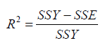
Where SSE (the sum of squares of residuals) and SSY
Adjusted R - square (adj-R2)
Since the number of parameters in the regression model
is not taken into account by R2, as R2 is monotonic increases,
the adjusted coefficient of multiple determination (Adj - R2)
has been suggested as an alternative criterion. The Adj - R2
method is similar to the method and it finds the best models
with the highest Adj- R2 within the range of sizes.
To determine this, we may calculate the adjusted Rsquare.
This is defined as
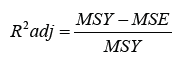
where MSY = SSY /( N −1) and MSE = SSE /(n − k) .
Mean Square Error MSE
The mean square error measures the variability of the
observed points around the estimated regression line, and
as such is an estimate of the error variance σ 2 . When using
as model selection tools, one would calculate the possible
subset of the predictor variables and then select the subset
corresponding to the smallest value of MSE to be included to
the final model.
It is defined as
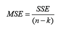
where SSE is again merely the sum squared error terms
and does not take account how many observations. The
smaller the value of MSE, the closer the predicted values
come to the real value of respond variables.
Mallows Statistics Cp
A measure that is quite widely used in model selection
is the Cp criterion measure, originally proposed by C.L. Mallows
(1973). It has the form:
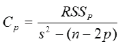
where RSSp residual sum of squares from a model containing
p parameters, p is the number of parameters in the
model including 0 β, s2 is the residual mean square from
the largest equation postulated containing all the X's, and
presumed to be a reliable unbiased estimate of the error
variance σ2.
R.W. Kennard (1971) has pointed out that Cp is closely
related to the adjusted Rp2 and Rp2 statistic. Let us consider
the relationship between adj- Rp2 or Rp2 & Cp.
Rp2 can be written as
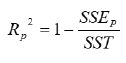
where SSEp being the error of squares and SST is the
total sum of squares.
The adjusted coefficient of multiple determination (Adj -
Rp2),
may also be considered as:
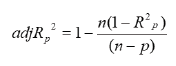
Rp2 and adjRp2 is used for model containing only p of
the K predictor variables. When the full model is used (all k
predictor variables included) the following notation is used:
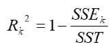
and the estimate of the error variance is then given as:
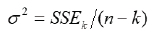
From equation (i) making SSEp the subject of the formula.
It follows that

Substitute this into Cp
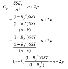
It is easily seen that Cp can be written as a function of the
multiple correlation coefficient. Making (1 − Rp2) the subject
of the formula from equation (3.7). It follows that in the relationship
between Cp and
adjR(p)2 we have
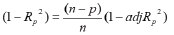
Then from
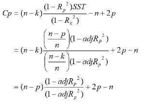
It is clear that there is a relationship between the adj-Rp2
or Rp2 and Cp statistics. In fact in both cases for each P the
minimum Cp and the maximum adj-Rp2 or Rp2 occur for the
same set of variables, although the P value of finally chosen
may of course differ. The factor (n − k) in the first equation
may cause decreases in minimum Cp values as P increases
although Rp2 is only slowly increasing. Several authors have
suggested using Cp as a criterion for choosing a model. We
look for model with a small Cp and P preferably we look for a
Cp close to P which means a small bias.
Forward Selection
In the forward selection procedure the analysis begins
with no explanatory (independent) variables in the regression
model. For each variable, a statistic called an F-statistic
(F -to-enter) is calculated; this F-statistic reflects the amount
of the variable’s contribution to explaining the behaviour
of the outcome (dependent) variable. The variable with the
highest value of the F - statistic (F-to-enter) is considered
for entry into the model. If the F -statistic is significant then
that variable is added to the model. If -statistic (F -to-enter)
is greater than 10 or more, then explonatory variables are
added to form a new current model. The forward selection
procedures are repeated until no additional explanatory
variables can be added [29-32].
Backward Elimination
The backward elimination method begins with the largest
regression, using all possible explanatory variables and
subsequently reduces the number of variables in the equation
until is reached in the equation to use. For each variable,
a statistic called an F -statistic (F-to-remove) is calculated.
The variable with the lowest value of the F-statistic
(F-to-remove) is considered for removal from the model. If
the -statistic is not significant then that variable is removed
from the model; if the F-statistic (F -to-remove) is 10 or less,
then explanatory variables are removed to arrive at a new
current model. The backward selection procedures are repeated
until none of the remaining explanatory variables can
be removed [33-39].
Stepwise Regression
Stepwise Regression is a combination of forward selection
and backward elimination. In stepwise selection which
can start with a full model, with the model containing no
predictors, or with a model containing some forced variables,
variables which have been eliminated can again be
considered for inclusion, and variables already included in
the model can be eliminated. It is important that the F-statistic
(F-to-remove) is defined to be greater than the F-statistic
(F-to-enter), otherwise the algorithm could enter and
delete the same variable at consecutive steps. Variables can
be forced to remain in the model and only the other variables
are considered for elimination or inclusion.
Akaike Information Criterion (AIC)
Akaike (1973) adopted the Kullback-Leibler definition
of information I(f;g), as a measure of discrepancy, or
asymmetrical distance, between a “true” model f and a proposed
model g, indexed on parameter vector Θ . Based on
large-sample theory, Akaike derived an estimator for I(f;g)
of the general form:

where the first term tends to decrease as more parameters
are added to the approximating family g(y/Θ) The second
term may be viewed as a penalty for over-parameterization.
Akaike Information Criterion (AIC)
Bayesian Information Criterion (BIC)
Bayesian information criterion (BIC) was introduced by
Schwartz in 1978. BIC is asymptotically consistent as a selection
criterion. That means, given a family of models including
the true model, the probability that BIC will select the correct
one approaches one as the sample size becomes large.
AIC does not have the above property. Instead, it tends to
choose more complex models as for small or moderate samples;
BIC often chooses models that are too simple, because
of its heavy penalty on complexity.
A model, which maximizes BIC is considered to be the
most appropriate model.

Where L is the maximum log likelihood, k is the number
of free parameters and n is the number of independent
(scalar) observation that contributes to likelihood. Model
selection here is carried out by trading off lack of fit against
complexity. A complex model with many parameters, having
large value in the complexity term, will not be selected unless
its fit is good enough to justify the extra complexity. The
number of parameters is the only dimension of complexity
that this method considers than AIC, BIC always provides
a model with a number of parameters no greater than that
chosen by AIC.
Methods
In this paper the data were partitioned into 13 sites and
models fitted independently to each site. This was partially
motivated during a personal discussion with Sir David Cox
of the University of Oxford, who suggested that the tumours
at different sites may in fact be different diseases, and therefore,
may require different models for the logit of the probabilities
of malignant tumours. The response variable indicated
the presence of either malignant or benign tumours and
is therefore a binary response. The task was now to model
the probability of a malignant tumour in terms of patient
age. The modern regression theory indicates that the logit of
these probabilities, rather than the probabilities themselves,
should be modelled either by a General Linear Model (GLM),
Generalized Additive Model (GAM) or a Kernel Smooth.
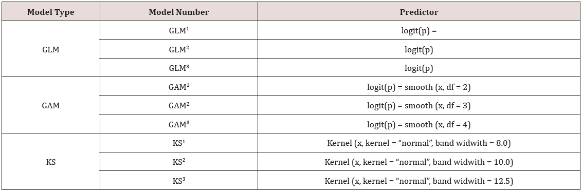
At each of the 13 sites, the logit of the probabilities was
modelled by increasingly flexible predictors namely: A GLM
using linear or quadratic predictors, a GAM with 2, 3, and
4 degrees of freedom and a Gaussian Kernel smooth using
various bandwidths, namely 8.0, 10.0 and 12.5. These are
summarised in Table 1. In order to select which of the above
model predictor combinations was the best at each site, we
applied the model selection criteria AIC, BIC and AICc. All
models were fitted using S-plus 4.0 for the purpose of assessing
the models in this study. The routines for computing
AIC, BIC and AICc in S-plus are given in Appendix 1 to 13.
The model selection criteria, AIC, BIC and AICc were computed
for each of the models described in Table 1 at each site.
The model with the smallest value of AIC, BIC and AICc was
then selected as the best model at a particular site. Because
the Kernel smooth is a non-parametric regression without
distributional assumption, it does not have a likelihood function
associated with it. Because of this, the model selection
criteria AIC, BIC and AICc, all of which require a likelihood,
cannot be computed. We have used Kernel estimators as a
non- parametric check on the best model selected from the
GLM’s and GAM’s.
Table 1: Table showing the predictors that were considered for each of the various models.
Results
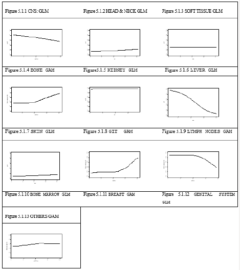
This section provides a detailed analysis of site 8 (Figure1)
and a summary of the best models that were fitted at
each of the best sites. This was done through presentation
and discussion of the fitted models using graphs (Figure 2)
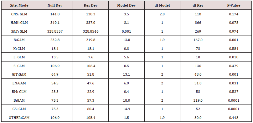
followed by the analysis of deviance for each of thse fitted
models as shown in Table 2. Detailed statistics for the other
sites are given in Appendix 1.
Figure 1: Comparison of the estimated probability model fitted at GIT.
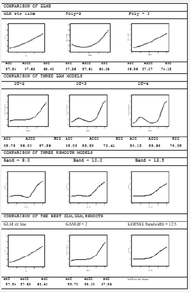
Figure 2: Graphs of estimated probabilities of malignant tumours for the best model at each of the13 sites using either a GLM or
a GAM.
Detailed Analysis of Site 8 (Genital Internal Track)
Consider the first row of model in Figure 2 which represents
the GLM using respectively a linear, quadratic and
cubic predictor i.e
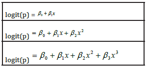
For these three models, using AIC, BIC and AICc as the
model selection criteria, the GAM with 2 degrees of freedom
was the selected model. In Figure 2 the first row provides a
comparison of the GLM’s using a linear, quadratic and cubic
predictor. Both the linear and cubic predictor appears to give
similar reasonable results. The quadratic predictor, however,
seems to have too much forced curvature in the left-hand
corner which appears to be contrary to medical experience.
The second row provides a comparison of GAM’s using 2,
3, and 4 degrees of freedom respectively. The models with
3 and 4 degrees of freedom appear to have too much force
curvature. The Gaussian Kernel smooth for bandwidth of 8.0
and 10.0 shows jubias curve that cannot reflect the probabilities
observed in real life. The third row provides a comparison
of the three final curves selected as the best fitted
model from the GLM, the GAM and the Kernel Smooth. Based
on the AIC, BIC and AICc criteria we have selected the GAM
with 2 degrees of freedom values that are listed below the
graph. It can be seen from the graph that although this has
the minimum value of AIC, it is highly constrained by linearity
of the predictor. The Kernel Smooth, however, is much
more flexible and therefore more able to follow the data. The
Kernel Smooth also seems to indicate that the logit may not
be linear.
Discussion
Central Nervous System (Figure 2). The graph conveys
that the probability of a malignant tumour starts from 80%
at birth and decreases to 50% at age 20. The majority of tumours
are malignant primitive neuroectodermal tumours
and there are few benign tumours. As the children become
older, the increase in astroeytic tumours remain few.ss The
model deviance is 3.5 on 2.0 degree of freedom with the
p=0.174 Therefore we concluded that the model is not significant
for the deviance. Head and Neck (Figure 2). It starts
from 10% for infants and increases to 20% for teens. The
majority of these tumours are benign haemangiomas and
lymphangionias.
Very few malignant tumours occur in this area. The model
deviance of 3.1 on 1 degree of freedom with a p= 0.078
which is not significant (Table 2). Therefore, the model is not
significant for reducing the deviance in head and neck. Soft
tissue (Figure 2) There is no change of the probability of a
malignant tumour from infants to late teens. The majority
of these tumours are benign, which it remains constant at
30%. Soft tissue sarcoma is rare. The commonest tumours
are lymphomas and haemangiomas. The model is not significantly
different from the null model of constant probability:
The model deviance is 0.001 on 1 degree of freedom with a
p= 0.974. Therefore, we concluded that the model is not significant
for the deviance. Bone (Figure 2) The probability of
a malignant tumour starts from 35% in early childhood and
remains constant until age 10 and then rises steeply during
the teens to 80% at age 20. Bone tumours are rare in infancy.
The sudden rise of the curve is caused by osteosarcoma
which is common between the ages of 10 to 20 years. The
model deviance is 13.0 on 1.9 degrees of freedom with a p=
0.001. Therefore, we concluded that the model explains a
significant portion of the deviance. Kidney (Figure 2) There
is a constant probability of malignant tumours close to 100%
over all ages from early childhood to age 20. The malignant
tumour are nephroblastomas. A few cases of congenital neuroblastic
nephroma were seen in malignant tumour. The
model is not significantly different from the null model of
constant probability: model deviance of 0.3 on 1 degree of
freedom with a p=0.584. Therefore, we concluded that the
model is not significant for the deviance.
Liver (Figure 2) The probability curve starts from 95%
for infants and steadily declines to 10% during the teen’s
years. The malignant tumours are Hepatoblast, which is
common before two years. This should explain the sudden
decline of the curve because malignant tumours are indeed
very high. The model deviance is 5.6 on 1 degree of freedom
with a p= 0.018. Therefore, we concluded that the model
explained a significant portion of deviance. Skin (Figure 2)
There is a constant probability of malignant tumours close
to 10% from early childhood to age 10 and this probability
steadily rises to 20% during teen years. A few malignant
tumours are present. The probability of contracting a malignant
tumour such as Kaporis sarcoma is rare in children.
The model deviance is 0.5 on 1 degree of freedom with a p=
0.479. Therefore, we concluded that the model does not explain
a significant portion of deviance. Genital Internal Track
(Figure 2) The graph conveys that the probability of a malignant
tumour starts from 15% for infants and remains constant
until age 13 and then rises steeply during the teens to
80% at age 20. This is consistent with the experience in medical
practice that the probability of contracting a malignant
tumour, at a very young age in the genital internal track is indeed very low and that there is a sudden rise of malignant
tumours around the age of 13.
The sudden rise in the 2nd decade is caused by lymphomas.
The model is strongly significant: The model deviance
is 13.1 on 2 degrees of freedom with a p= 0.001. Therefore,
we concluded that the model explains a significant portion
of deviance. Lymph Nodes (Figure2) The probability curve
starts from infants at 90% and remains constant until age
12 and then decreases during the teens to 40% at age 20.
Tumours at a very young age are lymph nodes which are
very high and there is a decrease of the probability curve at
the age of 13. The commonest tumours were lymphomas.
The model deviance is 6.9 on 2 degrees of freedom with a
p=0.031 Therefore we concluded that the model explains
a significant portion of deviance. Bone Marrow (Figure 2)
There is a constant probability of malignant tumours close to
100% from early childhood to age 20 years of age. This resonates
with the experience in medical practice that the probability
of contracting malignant tumours is lymphomas and
leukaemias that are found in malignant tumours. The model
is not significantly different from the null model of constant
probability. The model deviance is 0.4 on 1 degree of freedom
with a p= 0.527. Therefore, we concluded that the model
is not significant. Breast (Figure 2) The probability curve
starts from 90% at birth and steadily declines from malignant
to benign tumours and remains constant at 10% to late
teens. There was only one malignant tumour at four years.
This concurs with the experience in medical practice that the
probability of contracting a malignant tumour increases after
puberty and it is caused by fibroadenomas. The model is
strongly significant: The model deviance is 18.0 on 2 degrees
of freedom with a p= 0.0001. Therefore, we concluded that
the model explains a signify, can’t portion of deviance.
Genital System (Figure 2) There is a constant probability
of malignant tumours close to 40% from early childhood to
age 10 and slightly decreases to 2% during teen years. A few
malignant tumours are present. This is in line with the experience
found in medical practice that the probability of contracting
a malignant tumour is benign teratomas. The model
is not significant: The model deviance is 14.9 on 1 degree of
freedom with a p= 0.0001. Therefore, we concluded that the
model is not significant for the deviance in genital system.
Others (Figure 2) The graph indicates that the probability
of a malignant tumour starts from 45% for infants and remains
constant until age 13 and then rises steeply during the
teens to 50% until age 20. Malignant tumour for this group
of patients constitutes all those sites which did not have
enough cases. This should include sites where childhood malignamies
which are common, and they are rare. The model
deviance is 1.5 on 1.9 degrees of freedom with a p-value of
0.448 (Table 2) Therefore, we concluded that the model is
not significant for the deviance.
Table 2: Analysis of Deviance for best models at all sites.
Conclusion and Recommendation
The problem of model selection occurs almost everywhere
in statistics and we are facing more complicated data
sets in the study of complex diseases. Tools that are more
appropriate to the problem, more flexible to use, providing
a better description, should be adopted. Model selection by
AIC and BIC is one of these tools. We fitted a General Linear
Model, Generalized Additive Model or Kernel Smooth using
AIC and BIC model selections to the binary response to model
the probability of a malignant tumour in terms of patient
age. The probability of contracting a malignant tumour is
consistent with the experience in medical practice and is an
example of how model selections should be applied in practice.
The probability distribution of the response variable
was specified, and in this respect, a GAM is parametric.
In this sense they are more aptly named semi-parametric
models. A crucial step in applying GAMs is to select the
appropriate level of the ‘‘smoother’’ for a predictor. This is
best achieved by specifying the level of smoothing using the
concept of effective degrees of freedom. However, it is clear
that much work still has to be done, because we have found
that the Kernel smooth is a non-parametric regression which
is therefore does not have likelihood function associated
with it. Because of this the model selection criteria AIC and
BIC, both of which require a likelihood, cannot be computed.
We have used Kernel estimators as a non- parametric check
on the best model selected from the GLM’s and GAM’s.
Read More Current Trends on Biostatistics & Biometrics Please Click on Below Link https://lupine-publishers-biostatistics.blogspot.com/