Lupine Publishers | Journal of Current Trends on Biostatistics & Biometrics

Abstract
To identify the effect of risk factors on diabetic patients. a study was conducted among diabetic patients attending the outdoor at the Sheikh Zaid Hospital, Lahore. Data was collected by interviewing the patients using a structured questionnaire after the approval of synopsis. SPSS 23.0 was used for data entry and analysis. A sample of 100 respondents was selected by nonprobability convenient sampling. The risk factors were analyzed in a gender study of 100. Tabular form was used to represent the finding. Graphs shows the response of respondents. The Chi-Square test has been used to assess the statistical significance of risk factors for the diabetic patients. The check the normality of risk factors and then apply Mann-Whitney test to check the effect of each risk factor on diabetic patients w.r.t gender and marital status. The result found that in sheikh Zaid hospital patients only physical exercise, complications and environmental factors are affected in diabetic patients.
Keywords: Diabetic patient; questionnaire; risk factors; chi square test; mann whitney test
Introduction
Diabetes mellitus
The word “diabetes” stems from a Greek term for passing through, a reference to increased urination (polyuria), a common symptom of the disease. “Mellitus” is the Latin word for honeyed, a reference to glucose noted in the urine of diabetic patients. Diabetes mellitus is sometimes referred to as sugar diabetes but usually is simply called diabetes. Diabetes mellitus is a chronic disease caused by inherited or acquired deficiency of insulin production or resistance to action of the produced insulin. Diabetes occurs when the pancreas does not produce enough insulin (a hormone that regulates blood sugar) or alternatively, when the body cannot effectively use the insulin it produces. The overall risk of dying among people with diabetes is at least double the risk of their peers without diabetes (Setter et al., 2000). Insulin is more of an anabolic hormone rather than catabolic. Insufficient amounts of insulin or poor cellular response to insulin as well as defective insulin leads to improper handling of glucose by body cells or appropriate glucose storage in the liver and muscles. This ultimately leads to persistently high levels of blood glucose, poor protein synthesis, and other metabolic derangements. When there will be no insulin production or insulin become resistant then glucose will not be supply to the cells and remain as it is in the body. When it will not utilize by the cells then glucose level elevates in the body and cause hyperglycemic conditions in the body and the person is said to be diabetic. Following may be the reason of increased level of glucose in diabetic patients
- No production of insulin by pancreas
- Not enough insulin production that help in glucose supply to the cells
- Misfunctioning of insulin known as insulin resistance
The disease has been considered as one of the major health concerns worldwide today. The increase in incidence of diabetes in developing countries follows the trend of urbanization and lifestyle changes, perhaps most importantly diet [1]. Diabetes Mellitus is the common endocrine disease and affects nearly 10% of world population. At present, 347 million people worldwide have diabetes. In 2004, an estimated 3.4 million people died from consequences of fasting high blood sugar. A similar number of deaths have been estimated for 2010. More than 80% of diabetes deaths occur in low- and middle-income countries . Many experts continued to advise strict carbohydrate restriction, with the result that most people with diabetes adopted a high fat, low carbohydrate diet. Diabetes mellitus (DM) could be a risk factor for the development and progression of liver disease.
- Weight loss: Overly high blood sugar levels can also cause rapid weight loss, say 10 to 20 pounds over two or three months-but this is not a healthy weight loss. Because the insulin hormone is not getting glucose into the cells, where it can be used as energy, the body thinks it's starving and starts breaking down protein from the muscles as an alternate source of fuel.
- Hunger: Recessive pangs of hunger, another sign of diabetes, can come from sharp peaks and lows in blood sugar levels. When blood sugar levels plummet, the body thinks it has not been fed and craves more of the glucose that cells need to function.
- Slow healing: Infections, cuts, and bruises that do not heal quickly are another classic sign of diabetes. This usually happens because the blood vessels are being damaged by the excessive amounts of glucose traveling the veins and arteries. This makes it hard for blood-needed to facilitate healing-to reach different areas of the body.
- Increased urination, excessive thirst: If you need to urinate frequently-particularly if you often must get up at night to use the bathroom-it could be a symptom of diabetes. The kidneys kick into high gear to get rid of all that extra glucose in the blood, hence the urge to relieve yourself, sometimes several times during the night. The excessive thirst means your body is trying to replenish those lost fluids.
- Causes of diabetes: The causes of diabetes are complex and only partly understood. This disease is generally considered multifactorial, involving several predisposing conditions and risk factors. In many cases genetics, habits and environment may all contribute to a person’s diabetes. Weight and body type, Family medical history, Lack of physical activity, Carbohydrate intake, Chemical exposure, Smoking, Alcohol intake. This is blamed largely on the rise of obesity and the global spread of Western-style habits: physical inactivity along with a diet that is high in calories, processed carbohydrates, and saturated fats and insufficient in fiber rich whole foods. The aging of the population is also a factor. However, other factors, such as environment may also be contributing, because cases of autoimmune diabetes (type 1) are also becoming more common [2-10]. Experts are urging people to help stem this epidemic by getting regular exercise and controlling their diet and weight. Humans are not the only species that can develop diabetes. This disease also occurs in dogs, cats and other animals, as increasing numbers of pet owners are discovering.
Diabetic complications
The direct and indirect effects on the human vascular tree are the major source of morbidity and mortality in both type 1 and type 2 diabetes. Generally, the injurious effects of hyperglycemia are separated into macrovascular complications (coronary artery disease, peripheral arterial disease, and stroke) and microvascular complications (diabetic nephropathy, neuropathy, and retinopathy). More than half of all individuals with diabetes eventually develop neuropathy. Long-term metabolic complications of diabetes mellitus include retinopathy, nephropathy, peripheral neuropathy, amputations, and Charcot joints as well as autonomic neuropathy causing gastrointestinal, genitourinary, cardiovascular symptoms and sexual dysfunction. Diabetics are also at a greater risk atherosclerotic, cardiovascular, peripheral arterial and cerebrovascular disease. Hypertension and abnormalities of lipoprotein metabolism also accompany uncontrolled diabetes mellitus. These cardiovascular disorders are the leading cause of death in people with diabetes. Diabetes is the chief cause of end-stage renal disease, which requires treatment with dialysis or a kidney transplant. These include diabetic retinopathy, glaucoma and cataracts. Diabetes is a leading cause of visual impairment and blindness. This includes peripheral neuropathy, which often causes pain or numbness in the limbs, and autonomic neuropathy, which can impede digestion (gastroparesis) and contribute to sexual dysfunction and incontinence. Neuropathy may also impair hearing and other senses. Many studies have linked diabetes to increased risk of memory loss, dementia, Alzheimer’s disease and other cognitive deficits. Recently some researchers have suggested that Alzheimer’s disease might be “type 3 diabetes,” involving insulin resistance in the brain. Foot conditions and skin disorders, such as ulcers, make diabetes the leading cause of nontraumatic foot and leg amputations. People with diabetes are also prone to infections including periodontal disease, thrush, urinary tract infections and yeast infections [11-16]. Diabetes increases the risk of malignant tumors in the colon, pancreas, liver and several other organs. Conditions ranging from gout to osteoporosis to restless legs syndrome to myofascial pain syndrome are more common in diabetic patients than nondiabetics. Diabetes increases the risk of preeclampsia, miscarriage, stillbirth and birth defects. Many but not all the studies exploring connections between diabetes and mental illness have found increased rates of depression, anxiety and other psychological disorders in diabetic patients. In addition to chronic hyperglycemia, diabetic patients can experience acute episodes of hyperglycemia as well as hypoglycemia (low glucose).
Gestational diabetes
Gestational diabetes mellitus (GDM) is defined as any degree of glucose intolerance with onset or first recognition during pregnancy. The definition applies whether insulin or only diet modification is used for treatment and whether the condition persists after pregnancy. Approximately 7% of all pregnancies are complicated by GDM, resulting in more than 200,000 cases annually.
Type 1 diabetes
In type 1 diabetes, hyperglycemia occurs because of a complex disease process where genetic and environmental factors lead to an autoimmune response that remains to be fully elucidated. During this process, the pancreatic B-cells within the islets of Langerhans are destroyed, resulting in individuals with this condition relying essentially on exogenous insulin administration for survival, although a subgroup has significant residual C- peptide production. Type 1 diabetes is a disease in which the pancreas does not produce any insulin. Insulin is a hormone that helps your body to control the level of glucose (sugar) in your blood. Without insulin, glucose builds up in your blood instead of being used for energy. Your body produces glucose and gets glucose from foods like bread, potatoes, rice, pasta, milk, and fruit. An autoimmune disease in which the immune system mistakenly destroys the insulin-making beta cells of the pancreas. It typically develops more quickly than other forms of diabetes. It is usually diagnosed in children and adolescents, and sometimes in young adults. To survive, patients must administer insulin medication regularly. This form of diabetes previously encompassed by the terms insulin–dependent diabetes, Type 1 diabetes, or juvenile– onset diabetes, results from autoimmune mediated destruction of the beta cells of the pancreas. The rate of destruction is quite variable, being rapid in some individuals and slow in others. The rapidly progressive form is commonly observed in children, but also may occur in adults. The slowly progressive form generally occurs in adults and is sometimes referred to as latent autoimmune diabetes in adults (LADA) [17-26]. Markers of immune destruction, including islet cell autoantibodies, and/or autoantibodies to insulin, and autoantibodies to glutamic acid decarboxylase (GAD) are present in 85–90 % of individuals with Type 1 diabetes mellitus when fasting diabetic hyper glycaemia is initially detected.
Type 2 diabetes
Type 2 diabetes is the result of failure to produce sufficient insulin and insulin resistance. Elevated blood glucose levels are managed with reduced food intake, increased physical activity, and eventually oral medications or insulin. Type 2 diabetes is believed to affect more than 15 million adult Americans, 50% of whom are undiagnosed. It is typically diagnosed during adulthood. However, with the increasing incidence of childhood obesity and concurrent insulin resistance, the number of children diagnosed with type 2 diabetes has also increased worldwide Type 2 diabetes is Caused by insulin resistance in the liver and skeletal muscle, increased glucose production in the liver, over production of free fatty acids by fat cells and relative insulin deficiency. Insulin secretion can be decreases with gradual failure of beta cells.
Contributing factors of type 2 diabetes: Obesity, Age (onset of puberty is associated with increased insulin resistance) Lack of physical activity, Genetic predisposition, Racial/ethnic background (African American, Native American, Hispanic and Asian/Pacific Islander), Conditions associated with insulin resistance, (e.g., polycystic ovary syndrome).
Causes of type 2 diabetes: Obesity, Excess glucorticoid, Excess growth hormone, Gestational diabetes, Polycystic ovary disease, Lipodystrophy, Mutation of insulin receptor, Hemochromatosis, Blurry vision, Tingling or numbness. The most significant contributors to or causes of type 2 diabetes are diet and exercise. Obesity is a major risk-factor for diabetes.
Blurry vision: Having distorted vision and seeing floaters or occasional flashes of light are a direct result of high blood sugar levels. "Blurry vision is a refraction problem. Diabetes mellitus is group of metabolic disorders characterized by hyper glycemia, glycosuria and hyperlipemia”. In 2000 almost 177 million inhabitants of the world were affected by diabetes and in future (2025) predictable range of the people which are going to effect by the diabetes is 300 million. Type 2 diabetes is the type of diabetes in which insulin is produced but cells don’t take insulin for glucose uptake. Inactive sittings, fatness is the main cause of type 2 diabetes. Diabetes is a global problem, and its occurrence is continuously increasing in the world. Pakistan is at 7th rank in list of countries and it expected to have on 4th rank in future. Therefore, for research purpose diabetes is selected because the ratio of this disease is continuously increasing. Serum samples were collected from Sheik Zayed hospital Lahore because this hospital was nearer to Punjab University Lahore and have a separate diabetes department.
Methodology:
Study design: It was a cross-sectional study.
Setting: The Study was conducted at Diabetes Centre, Sheikh Zaid Hospital Lahore.
Selection of hospital: Shaikh Zayed Hospital is a tertiary care hospital located in Lahore, Punjab, Pakistan. It is attached with Shaikh Khalifa Bin Zayed Al-Nahyan Medical and Dental College as a teaching hospital and is part of Shaikh Zayed Medical Complex Lahore. And hospital is under Government of Pakistan. Their management will be very fine as compared other government hospitals. People believes that hospital is better than other so mostly people are coming in this hospital for their treatments so that why I use this hospital.
Target Population: All the patient came to the outpatient diabetes department of Sheikh Zaid Hospital Lahore. Who have Type 2 diabetes?
Duration of study: The duration of study was two months (02-05-2018 to 02-07-2018) after the approval of synopsis.
Sample Selection: Sample selection is one of the most vital steps for conducting a research. As the conclusion of the study is based on sample and all the inference are consequently referred to whole the population it should be a good representative to the target population.
Sampling technique: Non-probability convenient sampling technique was used for collection of data.
Sample size: 1000 cases were used in this study.
Data collection procedure: The success of the survey depends upon accuracy of the data collection. The correction of the accurate data depends upon the correct choice of survey method. After questionnaire, the next step was data collection. Face to face method was used for the collection of data keeping in mind the difficulty of locating the respondent after giving them the questionnaire. So, it was the best way to give the questionnaire to the respondent and be there for a while until the respondent fill and give it back. Respondent asks the purpose of the survey, meaning of the questions which they do not completely understand. Data were collected by suing a Performa/Questionnaire. The first part of the Performa contained information’s about the demographic characteristic of the patients while the second part contained information regarding risk factors of the disease. The collection of the accurate data depends upon the careful construction of a tool of data collection. There are some difficulties in field experience [27-34]. The respondent’s behavior was good, but some respondents refused to fill up the questionnaire. After explaining the objective of the study, they agreed to cooperate. Though at some places of the behavior of the respondents were not encouraging but it was a great experience overall.
- Inclusion criteria: The patient came to the outpatient diabetes department agreed to provide information.
- Exclusion criteria: Patients who are not agreeing to provide information.
Data Analysis:
Software package: Data were entered and analyzed by using SPSS (Statistical Package for Social Science) version 23.
Statistical Technique
- Descriptive Analysis: For descriptive of variables frequency were shown in tables. Charts and graphs were given for percentages in qualitative variables.
- Analytical Analysis: To find the risk variable of diabetes gender wise the current section is divided in the two main components.
- Bivariate Analysis
- Logistic Regression
Results
Figure 1: Shows the perecentage variation among the diabetic patients with various factors from figure 4.1.1 to 4.2.41.
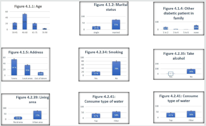
This study consists of 1000 subjects in which both male and female are included. There are 53 variables age, other diabetic patients in family, family members, address, marital status, gender, regarding follow doctor, type of meal, skip meal, gain weight, vision problem, wound problem, sugar fluctuation, social life, smoking, alcohol, alcohol frequently use, sanitary area, regularly use of medicine, fact of necessary exercise, fact of routine walk, daily walk, exercise, kind of exercise, time of exercise, day spend in exercise, walking time, Meals, hoteling, frequently of hoteling, use of fruits, use of milk, take care of yourself, loss weight, kidney problem, skin problem, regularly check sugar, sugar check time in a day, sugar record, sugar level, routine work, hobbies, effect of diabetes, industry area, industry type, living area, type of water, kind of medicine, use of vitamins, check-up, discuss problem with doctor, satisfaction from treatment. Figure 1 shows that out of 1000 respondents, 23(23.0%) persons have 30-45 age, 52(52.0%) persons have 46-60, 21(21.0%) persons have 61-75 and 4(4.0%) persons have 76-90. Among 23 persons who have the 30-45 age, the count (percentages) for male and female were 7(30.4%) and 16(69.6%) respectively and among 52 persons who have the 46-60 age, the count (percentages) for male and female were 16(30.8%) and 36(69.2%) respectively and among 21 persons who have 76-90 age , the count (percentages) for male and female were 4(100.0%) and 0(0.0%) respectively . Figure 1 shows that out of 1000 respondents, 25 (25.0%) persons have single while 75(75.0%) persons have married. Among 25 persons who are single , the count (percentages) for male and females were 11(44.0) and 14(56.0%) respectively and among 75 persons who are married, the count (percentages) for male and females were 28(37.3%) and 47(62.7%) respectively. Figure 1 shows that of out of 1000 respondents, 37(37.0%) persons have 1-5 family members, 47(47.0%) persons have 6-10 family members, 12(12.0%) have 11-15 family members and 4(4.0% have 16-20 family members. Among 37 persons have 1-5 family members, the count (percentages) for male and females were 18(49.6%) and 19(51.4%) respectively and among 47 persons have 6-10 family members, the count (percentages) for male and females were 19(40.4%) and 28 (59.6%) respectively and among 12 persons have 11-15 family members, the count (percentages) for male and females were 1(8.3%) and 11(91.7%) respectively and among 4 persons have 16-20 family members, the count (percentages) for male and females were 1(25.0%) and 3(75.0%). Figure 1 shows that of out of 1000 respondents, 34(34.0%) persons have 1-2 diabetic patient in family members, 8(8.0%) persons have 3-4 diabetic patient in family members, 3(3.0%) have 5-6 diabetic patient in family members and 55(55.0%) have no diabetic patient in family members. Among 34 persons have 1-2 diabetic patient in family members, the count (percentages) for male and females were 12(35.3%) and 22(64.7%) respectively and among 8 persons have 3-4 diabetic patient in family members, the count (percentages) for male and females were 0(0.0%) and 8(100.0%) respectively and among 55 persons have no diabetic patient in family members, the count (percentages) for male and females were 27(49.1%) and 28(50.9%) respectively [35-46]. Figure 1 shows that of out of 1000 respondents, 54(53.0%) persons address of towns, 3535.0%) persons have address of local areas and 11(11.0%) persons address out of Lahore. Among 54 persons address of towns, the count (percentages) for male and females were 20(37.0%) and 34(63.0%) respectively and among 35 persons address of local areas, the count (percentages) for male and females were 16(45.7%) and 19(54.3%) respectively and among 11 persons address of out of Lahore, the count (percentages) for male and females were 3(27.3%) and 8(72.7%) respectively Figure 1 shows that of out of 1000 respondents, 22(22.0%) persons that are doing smoking and 78(78.0%) persons that are not doing smoking. Among 22 that are doing smoking, the count (percentages) for male and female were 20(90.0%) and 2(9.1%) respectively and among 78 persons that are not doing smoking, the count (percentages) for males and females were 19(24.4%) and 59(75.6%) respectively Figure 1 shows that of out of 1000 respondents, 6(6.0%) persons that are taking alcohol and 94(94.0%) persons that are not taking alcohol. Among 6 that are taking alcohol, the count (percentages) for male and female were 6(100.0%) and 0(0.0%) respectively and among 94 persons that are not taking alcohol, the count (percentages) for males and females were 33(35.1%) and 61(64.5%) respectively Figure 1 shows that of out of 1000 respondents, 23(23.0%) persons that are living in rural area and 77(77.0%) persons that are living in urban area [47-53]. Among 23 that are living in rural area, the count (percentages) for male and female were 6(26.1%) and 17(73.9%) respectively and among 77 persons that are living in urban area, the count (percentages) for males and females were 33(42.9%) and 44(57.1%) respectively. Figure 2 shows that of out of 1000 respondents, 27(27.0%) persons that their area sanitary system is very good and 45(45.0%) persons that their area sanitary system is good and 17(17.0%) persons that there are a sanitary system is bad and 11(11.0%) persons that their area sanitary system is very bad. Among persons that their area sanitary system is very good, the count (percentages) for male and female were 4(14.8%) and 23(85.2%) respectively and among 45 persons that their area sanitary system is good, the count (percentages) for males and females were 27(60.0%) and 18(40.0%) respectively and among persons that there are a sanitary system is bad, the count (percentages) for male and female were 7(41.2%) and 10(58.8%) and 11 persons that their area sanitary system is very bad, the count (percentages) for male and female were 1(9.1) and 10(90.9%) respectively Figure 1 shows that of out of 1000 respondents, 42(42.0%) persons that consume tap water and 58(58.0%) persons that are consume filter water. Among 42 that are consume tap water, the count (percentages) for male and female were 15(35.7%) and 27(64.3%) respectively and among 58 persons that are consume filter water, the count (percentages) for males and females were 24(40.0%) and 36(60.0%) respectively. Figure 2 shows that of out of 1000 respondents, 25(25.0%) persons that are living in industrial area and 75(75.0%) persons that are not living in industrial area. Among 26 that are living in industrial area, the count (percentages) for male and female were 10(40.0%) and 15(60.0%) respectively and among 75 persons that are not living in industrial area, the count (percentages) for males and females were 29(38.7%) and 46(61.3%) respectively Figure 2 shows that of out of 1000 respondents, 80(80.0%) persons think that exercise is necessary for diabetic patients, 17(17.0%) persons thought that exercise is not necessary for diabetic patients and 3(3.0%) persons have no idea that exercise is suitable or not for diabetic patients. Among 80 persons think that the exercise is necessary for diabetic patients, the count (percentages) for male and females were 31(38.8%) and 49(61.3%) respectively and among 17 persons think that exercise is not necessary for diabetic patients, the count (percentages) for male and females were 6(35.3%) and 11(64.7%) respectively and among 3 persons don’t know that exercise is necessary for diabetic patients, the count (percentages) for male and females were 2(66.7%) and 1(33.3%) respectively. Figure 2 shows that of out of 1000 respondents, 88(88.0%) persons think that routine Walk is helpful for diabetic patients, 9(9.0%) persons think that walk is not helpful for diabetic patients and 3(3.0%) persons have no idea that walk is helpful or not. Among 88 persons think that the routine walk is helpful for diabetic patients, the count (percentages) for male and females were 32(36.4%) and 56(63.6%) respectively and among 9 persons think that routine is not helpful for diabetic patients, the count (percentages) for male and females were 5(55.6%) and 4(44.4%) respectively and among 3 persons don’t know that routine walk is helpful or not for diabetic patients, the count (percentages) for male and females were 2(66.7%) and 1(33.3%) respectively.
Figure 2: this shows percentage variation in pi charts form from 4.2.1 to 4.2.11.
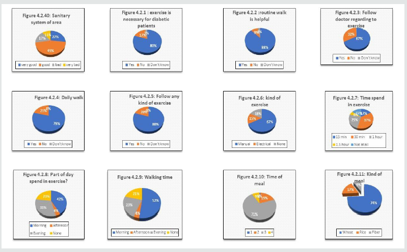
Figure 2 shows that of out of 1000 respondents, 67(67.0%) persons follow doctor regarding to exercise, 32(32.0%) persons do not follow doctor regarding to exercise, and 1(1.0%) persons don’t know about follow doctor regarding to exercise. Among 67 persons follow doctor regarding to exercise, the count (percentages) for male and females were 21(31.3%) and 46(68.7%) respectively and among 32 persons don’t follow doctor regarding to exercise, the count (percentages) for male and females were 18(56.3%) and 14(43.8%) respectively and among 1 persons don’t know about follow doctor regarding to exercise, the count (percentages) for male and females were 0(0.0%) and 1(100.0%) respectively Figure 2 shows that of out of 1000 respondents, 79(79.0%) persons go for daily walk, 21(21.0%) persons do not go for daily walk. Among 79 persons go for daily walk, the count (percentages) for male and females were 34(43.0%) and 45(57.0%) respectively and among 21 persons do not go for daily walk, the count (percentages) for male and females were 5(23.8%) and 16(76.2%) respectively. Figure 2 shows that of out of 1000 respondents, 80(80.0%) persons follow any kind of exercise, 20(20.0%) persons do not follow any kind of exercise. Among 80 persons follow any kind of exercise, the count (percentages) for male and females were 31(38.8%) and 49(61.3%) respectively and among 20 persons do not follow any kind of exercise, the count (percentages) for male and females were 8(40.0%) and 12(60.0%) respectively Figure 2 shows that of out of 1000 respondents, 67(67.0%) persons that follow manual exercise , 15(15.0%) persons that follow electrical exercise and 18(18.0) persons that don’t follow any manual or electrical exercise. Among 67 persons that follow manual exercise, the count (percentages) for male and females were 25(37.3%) and 42(62.7%) respectively and among 15 persons that follow electrical exercise, the count (percentages) for male and females were 6(40.0%) and 9(60.0%) respectively and among 18 persons don’t follow any manual or electrical exercise, the count (percentages) for male and females were 8(44.4%) and 10(55.6%) respectively Figure 2 shows that of out of 1000 respondents, 17(17.0%) persons that spend time in exercise 15 min, 37(37.0%) persons that spend time in exercise 30 min, 25(25.0) persons that spend time in exercise 1 hour , 6(6.0) persons that spend time in exercise 1.5 hour and 15(15.0) persons that spend no time on exercise. Among 17 persons that spend time in exercise 15 min, the count (percentages) for male and females were 3(17.6%) and 14(82.4%) respectively and among 37 persons that spend time in exercise 30 min, the count (percentages) for male and females were 19(51.4%) and 18(48.6%) respectively and among 25 persons that spend time in exercise 1 hour, the count (percentages) for male and females were 9(36.0%) and 16(64.0%) respectively and among 6 persons that spend time in exercise 1.5 hour, the count (percentages) for male and females were 1(16.7%) and 5(83.3%) respectively and among 15 persons that spend no time in exercise, the count (percentages) for male and females were 7(46.7%) and 8(53.3%) respectively
Figure 2 shows that of out of 1000 respondents, 42(42.0%) persons that spend morning in exercise, 4(4.0%) persons that spend afternoon in exercise, 31(31.0) persons that spend evening in exercise and 23(23.0%) persons spend no part of day in exercise. Among 42 persons that spend morning in exercise, the count (percentages) for male and females were 15(36.7%) and 27(64.3%) respectively and among 4 persons that spend afternoon in exercise, the count (percentages) for male and females were 2(50.0%) and 2(50.0%) respectively and among 31 persons that spend evening in exercise, the count (percentages) for male and females were 11(35.5%) and 20(64.5%) respectively and among 23 persons spend no part of day in exercise, the count (percentages) for male and females were 11(47.8%) and 12(52.2%) respectively. Figure 2 shows that of out of 1000 respondents, 52(52.0%) persons that spend morning for walk, 4(4.0%) persons that spend afternoon for walk, 23(23.0%) persons that spend evening for walk and 21(21.0%) persons spend no time for walk. Among 52 persons that spend morning for walk, the count (percentages) for male and females were 24(46.2%) and 28(53.8%) respectively and among 4 persons that spend afternoon for walk, the count (percentages) for male and females were 1(25.0%) and 3(75.0%) respectively and among 23 persons that spend evening for walk, the count (percentages) for male and females were 8(39.1%) and 14(60.9%) respectively and among 23 persons spend no time for walk, the count (percentages) for male and females were 5(23.8%) and 16(76.2%) respectively. Figure 2 shows that of out of 1000 respondents, 1(1.0%) persons that 1 time take meal in day, 19(19.0%) persons that 2 times take meal in a day, 71(71.0%) persons that 3 times take meal in a day, and 9(9.0%) persons that 4 times take meal in a day. Among 1 persons that 1 time take meal in a day, the count (percentages) for male and females were 0(0.0%) and 1(100.0%) respectively and among 19 persons that 2 times take meal in a day, the count (percentages) for male and females were 8(42.1%) and 11(57.9%) respectively and among 71 persons that 3 times take meal in a day, the count (percentages) for male and females were 25(35.2%) and 46(64.8%) respectively and among 9 persons that 4 times take meal in a day, the count (percentages) for male and females were 6(39.0%) and 3(33.3%) respectively. Figure 2 shows that of out of 1000 respondents, 74(74.0%) persons that use wheat in meal, 17(17.0%) persons that use rice in meal and 9(9.0%) persons that use fiber in meal. Among 74 persons that use wheat in meal, the count (percentages) for male and females were 33(44.6%) and 41(55.4%) respectively and among 17 persons that use rice in meal, the count (percentages) for male and females were 2(11.8%) and 15(88.2%) respectively and among 9 persons that use fiber in meal, the count (percentages) for male and females were 4(44.4%) and 5(55.6%) respectively. Figure 3 shows that of out of 1000 respondents, 37(37.0%) persons that go out for meal, 63(63.0%) persons that do not go out for meal. Among 37 persons that go out for meal, the count (percentages) for male and females were 15(40.5%) and 22(59.5%) respectively and among 63 persons that not go for meal, the count (percentages) for male and females were 24(38.%) and 39(61.9%) respectively .
Figure 3 shows that of out of 1000 respondents, 64(64.0%) persons that never go out for meal, 23(23.0%) persons that sometimes go out for meal, 8(8.0%) persons that normally go out for meal, and 5(5.0%) persons that have frequently go out for meal. Among 64 persons that never go out for meal, the count (percentages) for male and females were 25(39.1%) and 39(60.9%) respectively and among 23 persons that sometimes go out for meal, the count (percentages) for male and females were 7(30.4%) and 16(69.6%) respectively and among 8 persons that normally go out for meal, the count (percentages) for males and females were 5(62.5%) and 3(37.5%) respectively and among 5 persons that frequently go out for meal, the count (percentages) for male and female were 2(40.0%) and 3(60.0%). Figure 3 shows that of out of 1000 respondents, 41(41.0%) persons that regularly use of fruit, 20(20.0%) persons that are not use of fruit, 39(39.0%) persons that sometimes use the fruits. Among 41 persons that regularly use of fruit, the count (percentages) for male and females were 16(39.0%) and 25(61.0%) respectively and among 20 persons that are not use of fruit, the count (percentages) for male and females were 7(35.0%) and 13(65.0%) respectively and among 39 persons that sometime use of fruit, the count (percentages) for males and females were 16(41.0%) and 23(59.0%) respectively Figure 3 shows that of out of 1000 respondents, 48(48.0%) persons that regularly use of milk, 18(18.0%) persons that are not use of milk, 34(34.0%) persons that sometimes use the milk. Among 48 persons that regularly use of milk, the count (percentages) for male and females were 21(43.8%) and 27(56.3%) respectively and among 18 persons that are not use of milk, the count (percentages) for males and females were 4(22.2%) and 14(77.8%) respectively and among 34 persons that sometime use of milk, the count (percentages) for males and females were 14(41.2%) and 20(58.8%) respectively Figure 3 shows that of out of 1000 respondents, 37(37.0%) persons that skip their meal, 34(34.0%) persons that are not skip their meal, 29(29.0%) persons that response is don’t know means that persons have not in mind that they skip meal or not in routine. Among 37 persons that skip their meal, the count (percentages) for male and females were 7(18.9%) and 30(81.1%) respectively and among 34 persons that are not skip their meal, the count (percentages) for males and females were 19(55.9%) and 15(44.1%) respectively and among 29 persons that have not in mind that they skip meal or not in routine, the count (percentages) for males and females were 13(44.8%) and 16(55.2%) respectively.
Figure 3: This also shows the percentage variation in pi chart form from 4.2.12. to 4.2.40.
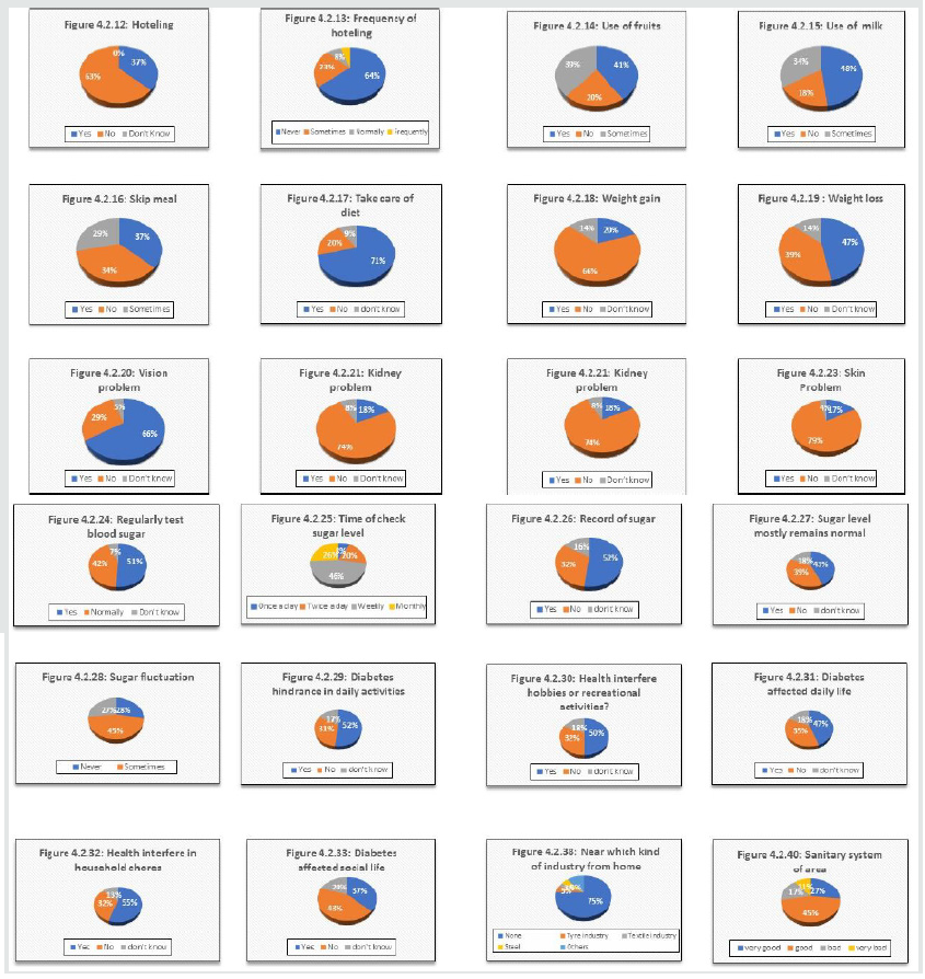
Figure 3 shows that of out of 1000 respondents, 71(71.0%) persons that take of their diet, 20(20.0%) persons that are not take of their diet, 9(9.0%) persons that response is don’t know means that persons have not in mind that they take of diet or not. Among 71 persons that skip their meal, the count (percentages) for male and females were 25(35.2%) and 46(64.8%) respectively and among 20 persons that are not take of their diet, the count (percentages) for males and females were 11(55.0%) and 9(45.0%) respectively and among 9 persons that have not in mind that they take of their diet or not, the count (percentages) for males and females were 3(33.3%) and 6(66.7%) respectively. Figure 3 shows that of out of 1000 respondents, 20(20.0%) persons that weight gain, 66(66.0%) persons that not weight gain, 14(14.0%) persons that response is don’t know means that persons have not know that about their weight that gain or not. Among 20 persons that gain weight, the count (percentages) for male and females were 2(10.0%) and 18(90.0%) respectively and among 66 persons that are not gain weight, the count (percentages) for males and females were 31(47.0%) and 35(53.0%) respectively and among 14 persons that don’t know that weight gain or not, the count (percentages) for males and females were 6(42.9%) and 8(57.1%) respectively. Figure 3 shows that of out of 1000 respondents, 47(47.0%) persons that weight loss, 39(39.0%) persons that not weight loss, 14(14.0%) persons that response is don’t know means that persons don’t know that about their weight that loss or not. Among 47 persons that loss weight, the count (percentages) for male and females were 18(38.3%) and 29(61.7%) respectively and among 39 persons that are not lose weight, the count (percentages) for males and females were 15(38.5%) and 24(61.5%) respectively and among 14 persons that don’t know that weight gain or not, the count (percentages) for males and females were 6(42.9%) and 8(57.1%) respectively Figure 3 shows that of out of 1000 respondents, 66(66.0%) persons that have vision problem, 29(29.0%) persons that have no vision problem and 5(5.0%) persons that response is don’t know means that persons don’t know that about their vision problem. Among 66 persons that have vision problem, the count (percentages) for male and females were 18(27.3%) and 48(72.2%) respectively and among 29 persons that have no vision problem, the count (percentages) for males and females were 17(58.6%) and 12(41.4%) respectively and among 5 persons that don’t know about their vision problem, the count (percentages) for males and females were 4(80.0%) and 1(20.0%) respectively. Figure 3 shows that of out of 1000 respondents, 18(18.0%) persons that have kidney problem, 74(74.0%) persons that have no kidney problem and 8(8.0%) persons that response is don’t know means that persons don’t know that about their kidney problem. Among 18 persons that have kidney problem, the count (percentages) for male and females were 4(22.2%) and 14(77.8%) respectively and among 74 persons that have no kidney problem, the count (percentages) for males and females were 30(40.5%) and 44(59.5%) respectively and among 8 persons that don’t know about their kidney problem, the count (percentages) for males and females were 5(62.5%) and 3(37.5%) respectively. Figure 3 shows that of out of 1000 respondents, 36(36.0%) persons that have wound healing problem, 56(56.0%) persons that have no wound healing problem and (8.0%) persons that response is don’t know means that persons don’t know that about their wound healing problem. Among 36 persons that have wound healing problem, the count (percentages) for male and females were 5(13.9%) and 31(86.1%) respectively and among 56 persons that have no wound healing problem, the count (percentages) for males and females were 29(51.8%) and 27(48.2%) respectively and among 8 persons that don’t know about their wound healing, the count (percentages) for males and females were 5(62.5%) and 3(37.5%) respectively.
Figure 3 shows that of out of 1000 respondents, 17(17.0%) persons that have skin problem, 79(79.0%) persons that have no skin problem and 4(4.0%) persons that response is don’t know means that persons don’t know that about their skin problem. Among 17 persons that have skin problem, the count (percentages) for male and females were 5(29.4%) and 12(70.6%) respectively and among 79 persons that have no skin problem, the count (percentages) for males and females were 32(40.5%) and 47(59.5%) respectively and among 4 persons that don’t know about their skin problem, the count (percentages) for males and females were 2(50.0%) and 2(20.0%) respectively Figure 3 shows that of out of 1000 respondents, 51(51.0%) persons check their sugar level regularly, 42(42.0%) persons that are not check their sugar level regularly and 7(7.0%) persons that response is don’t know means that persons don’t know that check their sugar level regularly. Among 51 persons that check their sugar level regularly, the count (percentages) for male and females were 15(29.4%) and 36(70.6%) respectively and among 42 persons that are not check their sugar level regularly, the count (percentages) for males and females were 22(52.4%) and 20(47.6%) respectively and among 7 persons that don’t know about check their sugar level regularly, the count (percentages) for males and females were 2(528.6%) and 5(71.4%) respectively Figure 3 shows that of out of 1000 respondents, 8(8.0%) persons check their sugar level once a day, 20(20.0%) persons that check their sugar level twice a day, 46(46.0%) persons that check their sugar level weekly and 8(8.0%) that check their sugar level monthly. Among 8 persons that check their sugar level once a day, the count (percentages) for male and female were 4(50.0%) and 4(50.0%) respectively and among 20 persons that check their sugar level twice a day, the count (percentages) for male and female were 7(35.0%) and 13(65.0%) respectively and among 46 persons that check their sugar level weekly, the count (percentages) for male and female were 20(43.5%) and 26(56.5%) respectively and among 8 person that check their sugar level monthly, the count(percentages) for male and female were 8(30.8%) and 18(69.2%) respectively. Figure 3 shows that of out of 1000 respondents, 52(52.0%) persons record their sugar level , 32(32.0%) persons that are not record their sugar level and 16(16.0%) persons that response is don’t know means that have not in mind that record their sugar level. Among 52 persons that record their sugar level, the count (percentages) for male and female were 19(36.5%) and 33(63.5%) respectively and among 32 persons that are not record their sugar level, the count (percentages) for males and females were 16(50.0%) and 16(50.0%) respectively and among 16 persons that don’t know means that have not in mind that record their sugar level, the count (percentages) for male and female were 4(25.0%) and 12(75.0%) respectively. Figure 3 shows that of out of 1000 respondents, 43(43.0%) persons mostly their sugar level remain normal , 39(39.0%) persons that are not their sugar level remain normal and 18(18.0%) persons that response is don’t know means that have not in mind that their sugar level remain normal. Among 43 persons that their sugar level remain normal, the count (percentages) for male and female were 18(41.9%) and 25(58.1%) respectively and among 39 persons that are not their sugar level remain normal, the count (percentages) for males and females were 14(35.9%) and 25(64.1%) respectively and among 18 persons that don’t know means that have not in mind that their sugar level remain normal, the count (percentages) for male and female were 7(38.9%) and 11(61.1%) respectively. Figure 3 shows that of out of 1000 respondents, 28(28.0%) persons never fluctuate their sugar level, 45(45.0%) persons sometimes fluctuate their sugar level and 27(27.0%) persons every time fluctuate their sugar level Among 28 persons never fluctuate their sugar level, the count (percentages) for male and female were 16(57.1%) and 12(42.9%) respectively and among 45 persons sometimes fluctuate their sugar level, the count (percentages) for males and females were 18(40.0%) and 27(60.0%) respectively and among 27 persons that every time fluctuate their sugar level, the count (percentages) for male and female were 5(18.5%) and 22(81.5%) respectively.
Figure 3 shows that of out of 1000 respondents, 52(52.0%) persons that agree that diabetes hindrance in daily activities, 31(31.0%) persons that not agree that diabetes hindrance in daily activities and 17(17.0%) persons that response answer in don’t know means they have no idea that diabetes hindrance in daily activities. Among 52 that agree that diabetes hindrance in daily activities, the count (percentages) for male and female were 20(38.5%) and 32(61.5%) respectively and among 31 persons that not agree that diabetes hindrance in daily activities, the count (percentages) for males and females were 11(35.5%) and 20(64.5%) respectively and among 17 persons that response answer in don’t know means they have no idea that diabetes hindrance in daily activities, the count (percentages) for male and female were 8(47.1%) and 9(53.9%) respectively. Figure 3 shows that of out of 1000 respondents, 50(50.0%) persons that agree that health interfere hobbies or recreational activities, 32(32.0%) persons that not agree that health interfere hobbies or recreational activities and 18(18.0%) persons that response answer in don’t know means they have no idea that health interfere hobbies or recreational activities. Among 50 that agree that health interfere hobbies or recreational activities, the count (percentages) for male and female were 16(32.0%) and 34(68.0%) respectively and among 32 persons that not agree that health interfere hobbies or recreational activities, the count (percentages) for males and females were 16(50.0%) and 16(50.0%) respectively and among 18 persons that response answer in don’t know means they have no idea that health interfere hobbies or recreational activities, the count (percentages) for male and female were 7(38.9%) and 11(61.1%) respectively. Figure 3 shows that of out of 1000 respondents, 47(47.0%) persons that agree that diabetes affected daily life, 35(35.0%) persons that not agree that diabetes affected daily life and 18(18.0%) persons that response answer in don’t know means they have no idea that diabetes affected daily life. Among 47 that agree that diabetes affected daily life, the count (percentages) for male and female were 15(31.9%) and 32(68.1%) respectively and among 35 persons that not agree that diabetes affected daily life, the count (percentages) for males and females were 17(48.6%) and 18(51.4%) respectively and among 18 persons that response answer in don’t know means they have no idea that health diabetes affected daily life, the count (percentages) for male and female were 7(38.9%) and 11(61.1%) respectively. Figure 3 shows that of out of 1000 respondents, 55(55.0%) persons that agree that health interfere in household chores, 32(32.0%) persons that not agree that health interfere in household chores and 13(13.0%) persons that response answer in don’t know means they have no idea that health interfere in household chores. Among 55 that agree that health interfere in household chores, the count (percentages) for male and female were 16(29.1%) and 39(70.9%) respectively and among 32 persons that not agree that health interfere in household chores, the count (percentages) for males and females were 16(50.0%) and 16(50.0%) respectively and among 13 persons that response answer in don’t know means they have no idea that health interfere in household chores, the count (percentages) for male and female were 7(53.8%) and 6(46.2%) respective. Figure 3 shows that of out of 1000 respondents, 37(37.0%) persons that agree that diabetes affected social life, 43(43.0%) persons that not agree that diabetes affected social life and 20(20.0%) persons that response answer in don’t know means they have no idea that diabetes affected social life. Among 37 that agree that diabetes affected social life, the count (percentages) for male and female were 6(16.2%) and 31(83.8%) respectively and among 43 persons that not agree that diabetes affected social life, the count (percentages) for males and females were 26(60.5%) and 17(39.5%) respectively and among 20 persons that response answer in don’t know means they have no idea that health diabetes affected social life, the count (percentages) for male and female were 7(35.0%) and 13(65.0%) respectively.
Figure 3 shows that of out of 1000 respondents, 0(0.0%) persons that are taking alcohol daily and 2(2.0%) persons that are taking alcohol weekly and 5(5.0%) persons that are taking alcohol monthly and 93(93.0%) persons are taking no alcohol. Among 0 that are taking alcohol daily, the count (percentages) for male and female were 0(0.0%) and 0(0.0%) respectively and among 2 persons that are taking alcohol weekly, the count (percentages) for males and females were 2(100%) and 0(0.0%) respectively and among 5 persons that are taking alcohol monthly, the count (percentages) for male and female were 4(80.0) and 1(20.0) and 93 persons that are not taking alcohol, the count (percentages) for male and female were 33(35.5) and 60(64.5) respectively. Figure 3 shows that of out of 1000 respondents, 75(75.0%) persons that are living in non- industrial area and 5(5.0%) persons that are living near the tyre industry and 3(3.0%) persons that are living near the textile industry and 5(5.0%) persons that are living near the steel mill and 12(12.0%) persons are living near the other industries. Among 75 that are living in non- industrial area, the count (percentages) for male and female were 29(38.7%) and 46(61.3%) respectively and among 5 persons that are living near the tyre industry, the count (percentages) for males and females were 3(60.0%) and 2(40.0%) respectively and among 3 persons that are living near the textile industry, the count (percentages) for male and female were 2(66.7%) and 1(33.3%) and 5 persons that are living near the steel mill, the count (percentages) for male and female were 1(20.0) and 4(80.0%) respectively and among 12 persons are living near the other industries, the count (percentages) for male and female were 4(33.3) and 8(66.7%) respectively. Figure 3 shows that of out of 1000 respondents, 27(27.0%) persons that their area sanitary system is very good and 45(45.0%) persons that their area sanitary system is good and 17(17.0%) persons that there area sanitary system is bad and 11(11.0%) persons that their area sanitary system is very bad. Among persons that their area sanitary system is very good, the count (percentages) for male and female were 4(14.8%) and 23(85.2%) respectively and among 45 persons that their area sanitary system is good, the count (percentages) for males and females were 27(60.0%) and 18(40.0%) respectively and among persons that there area sanitary system is bad, the count (percentages) for male and female were 7(41.2%) and 10(58.8%) and 11 persons that their area sanitary system is very bad, the count (percentages) for male and female were 1(9.1) and 10(90.9%) respectively. Figure 3 shows that of out of 1000 respondents, 60(60.0%) persons that taking pills in medicine, 20(20.0%) persons that are taking insulin in medicine and 20(20.0%) persons that taking combination of pills and insulin in medicine. Among 60 persons that taking pills in medicine, the count (percentages) for male and female were 24(41.4%) and 34(58.6%) respectively and among 20 persons that are taking insulin in medicine, the count (percentages) for males and females were 24(40.0%) and 36(60.0%) respectively and among 20 persons that taking combination of pills and insulin in medicine, the count (percentages) for male and female were 5(25.0%) and 15(75.0%) respectively.
Figure 3 shows that of out of 1000 respondents, 77(77.0%) persons that taking medicine regularly, 17(17.0%) persons that are not taking medicine and 6(6.0%) persons that miss sometime medicine. Among 77 persons that taking medicine regularly, the count (percentages) for male and female were 25(32.5%) and 52(67.5%) respectively and among 17 %) persons that are not taking medicine, the count (percentages) for males and females were 10(58.8%) and 7(41.2%) respectively and among 6 persons that miss sometime medicine, the count (percentages) for male and female were 4(66.7%) and 2(33.3%) respectively. Figure 3 shows that of out of 1000 respondents, 56(56.0%) persons that use of vitamins or supplements, 43(43.0%) persons that are not use of vitamins or supplements and 1(1.0%) persons that sometime use of vitamins or supplements. Among 56 that use of vitamins or supplements, the count (percentages) for male and female were 20(35.7%) and 36(64.3%) respectively and 43 persons that are not use of vitamins or supplements, the count (percentages) for males and females were 18(41.9%) and 25(58.1%) respectively among 1 persons that sometime use of vitamins or supplements, the count (percentages) for males and females were 1(100.0%) and 0(0.0%) respectively . Figure 3 shows that of out of 1000 respondents, 5(5.0%) persons that meet their doctor weekly, 70(70.0%) persons that meet their doctor monthly and 25(25.0%) persons that meet their doctor yearly. Among 5 that persons that meet their doctor weekly, the count (percentages) for male and female were 2(40.0%) and 3(60.0%) respectively and 70 persons that meet their doctor monthly, the count (percentages) for males and females were 28(40.0%) and 42(60.0%) respectively among persons that meet their doctor yearly, the count (percentages) for males and females were 9(36.0%) and 16(64.0%) respectively . Figure 3 shows that of out of 1000 respondents, 86(86.0%) persons that discuss problem in detail with doctor, 6(6.0%) persons that are not discuss problem in detail with doctor and 8(8.0%) persons that answer is don’t know means they don’t want to share that discuss in detail with doctor or not. Among 86 persons that discuss problem in detail with doctor, the count (percentages) for male and female were 34(39.5%) and 52(60.5%) respectively and among 6%) persons that are not discuss problem in detail with doctor, the count (percentages) for males and females were 2(33.3%) and 4(66.7%) respectively and among 8 persons that answer is don’t know means they don’t want to share that discuss in detail with doctor or not, the count (percentages) for male and female were 3(37.5%) and 5(62.5%) respectively.
Figure 3 shows that of out of 1000 respondents, 78(78.0%) persons that satisfied with their treatment, 12(12.0%) persons that are not satisfied with their treatment and 10(10.0%) persons that response is don’t know means they don’t want to share that are satisfied or not. Among 78 persons that satisfied with their treatment, the count (percentages) for male and female were 28(35.9%) and 50(64.1%) respectively and among 12 persons that are not satisfied with their treatment, the count (percentages) for males and females were 6(50.0%) and 6(50.0%) respectively and among 10 persons that response is don’t know means they don’t want to share that are satisfied or not, the count (percentages) for male and female were 5(50.0%) and 5(50.0%) respectively
Descriptive Analysis
In this section the frequency and percentages of the demographic, different variable of diabetes will be discussed with respect to diabetes gender. We will discuss here the frequency and percentages of demographic variables There are 1000 subjects. The debate of the results will base on the frequency, percentages.
Discussion
There were 39 males and 61 female’s people in sample of 1000. Percentage of male persons=39.0%, Percentage of female persons=61.0%. Out of 1000 respondents the number(percentage) of marital status in single and married group was 25(25.0%) and 75(75.0%) respectively. Out of 1000 respondents the number(percentage) of family members in 1-5, 6-10, 11-15 and 16-20 group was 37(37.0%),47(47.0%),12(12.0%) and 4(4.0%). Out of 1000 respondents the number(percentage) of other diabetic patient in family in 1-2, 3-4, 5-6 and No group was 34(34.0%), 8(8.0%), 3(3.0%) and 55(55.0%) respectively. Out of 1000 respondents the number(percentage) of Persons address in towns, local areas and out of Lahore group was 54(54.0%), 35(35.0%) and 11(11.0%) respectively. Out of 1000 respondents the number(percentage) of persons that following any exercise in yes and no group was 80(80.0%) and 20(20.0%) respectively. Out of 1000 respondents the number(percentage) of Persons that have skin problem after diabetes in yes, no and don’t know group was 17(17.0%), 79(79.0%) and 4(4.0%) respectively. Out of 1000 respondents the number(percentage) of Persons that have wound healing problem after diabetes in yes, no and don’t know group was 36(36.0%), 56(56.0%) and 8(8.0%) respectively. Out of 1000 respondents the number(percentage) of Persons that have kidney problem after diabetes in yes, no and don’t know group was 18(18.0%), 74(74.0%) and 8(8.0%) respectively. Out of 1000 respondents the number(percentage) of Persons that have vision problem after diabetes in yes, no and don’t know group was 66(66.0%), 29(29.0%) and 5(5.0%) respectively. Out of 1000 respondents the number(percentage) of Persons have weight loss after diabetes in yes, no and don’t know group was 47(47.0%), 39(39.0%) and 14(14.0%) respectively. Out of 1000 respondents the number(percentage) of Persons have weight gain after diabetes in yes, no and don’t know group was 20(20.0%), 66(66.0%) and 16(16.0%) respectively. Out of 1000 respondents the number(percentage) of Persons that hoteling in yes and no group was 37(37.0%), 63(63.0%) respectively.
Out of 1000 respondents the number(percentage) of Persons that taking kind of meal in Wheat, Rice and Fiber group was 84(84.0%), 13(13.0%) and 3(3.0%) respectively. Out of 1000 respondents the number(percentage) of Persons that number of taken meal in a day in 1, 2, 3 and 4 group were 1(1.0%) 19(19.0%), 71(71.0%) and 9(9.0%) respectively. Out of 1000 respondents the number(percentage) of Persons that are frequently hoteling in Never, Sometimes, Normally and Frequently group was 64(64.0%), 23(23.0%) ,8(8.0%) and 5(5.0%) respectively. Out of 1000 respondents the number(percentage) of Persons that regularly test their blood sugar level in yes, no and don’t know group was 51(51.0%), 42(42.0%) and 7(7.0%) respectively. Out of 1000 respondents the number(percentage) of Persons that check their sugar in a day in once a day, twice a day, Weekly and Monthly group was 8(8.08%), 20(20.0%), 46(46.0) and 26(26.0%) respectively. Out of 1000 respondents the number(percentage) of Persons that fluctuate their sugar in never, sometimes and every time group was 28(28.0%), 45(45.0%), 27(27.0) respectively. Out of 1000 respondents the number(percentage) of Persons living in industrial area Yes and NO group was 25(25.0%) and 75(75.0%) respectively. Out of 100 respondents the number(percentage) of Persons living near the which factory in None, Tyre industry, Textile industry, Steel and Others group was 75(75.0%), 5(5.0%), 3(3.0%), 5(5.0%), 12(12.0%) respectively .Out of 1000 respondents the number(percentage) of Persons living area in rural area and urban area group was 23(23.0%) and 77(77.0%) respectively.
Out of 1000 respondents the number(percentage) of Persons satisfied their sanitary system in very good, good, bad and very bad group was 27(27.0%), 45(45.0%), 17(17.0%) and 11(11.0%) respectively .Out of 1000 respondents the number(percentage) of Persons that use which type of water in tap and filter group was 42(42.0%), 58(58.0%) respectively. Out of 1000 respondents the number(percentage) of Persons that taking kind of medicine pills, insulin and combination group was 60(60.0%), 20(20.0%) and 20(20.0%) respectively. Out of 1000 respondents the number(percentage) of Persons that regularly take medicine in yes, no and miss sometimes group was 77(77.0%), 17(17.0%) and 6(6.0%) respectively. Out of 1000 respondents the number(percentage) of Persons that are used vitamin or supplements in yes, no and sometime group was 56(56.0%), 43(43.0%) and 1(1.0%) respectively. Out of 1000 respondents the number(percentage) of Persons that meet their doctor in Weekly, Monthly, and yearly group was 5(5.0%), 70(70.0%) and 25(25.0%) respectively. Out of 1000 respondents the number(percentage) of Persons take alcohol in yes and no group was 6(6.0%) and 94(94.0%). Out of 1000 respondents the number(percentage) of Persons smoking in yes and no group was 22(22.0%) and 78(78.0%). Out of 1000 respondents the number(percentage) of Persons that are going for daily walk in yes, no and do not know group was 79(79.0%), 21(21.0%) respectively.
Out of 1000 respondents the number(percentage) of Persons that think the exercise is necessary for diabetic patients in yes, no and do not know group was 80(80.0%), 17(17.0%) and 3(3.0%) respectively. Out of 1000 respondents the number(percentage) of Persons that think routine walk is helpful for diabetic patients in yes, no and do not know group was 88(88.0%), 9(9.0%) and 3(3.0%) respectively. Out of 1000 respondents the number(percentage) of Persons follow doctor regarding exercise in yes, no and don’t know group was 67(67.0%), 32(32.0%) and 1(1.0%) respectively Out of 1000 respondents the number(percentage) of Persons that take proper fruit in yes, no and sometime group was 41(41.0%), 20(20.0%) and 39(39.0%) respectively. Out of 1000 respondents the number(percentage) of Persons that take milk regularly in yes, no, and sometime group was 48(48.0%), 43(43.0%) and 34(34.0%) respectively. Out of 1000 respondents the number(percentage) of Persons that skip their meal in yes, no and sometime group was 37(37.0%), 34(34.0%) and 29(29.0%) respectively. Out of 1000 respondents the number(percentage) of Persons that take care of their diet in yes, no and don’t know group was 71(71.0%), 20(20.0%) and 9(9.0%) respectively. Out of 1000 respondents the number(percentage) of Persons that affected their daily life from diabetes in yes, no and don’t know group was 47(47.0%), 35(35.0%) and 18(18.0%) respectively. Out of 1000 respondents the number(percentage) of Persons that their household chores affected form health in yes, no and don’t know group was 55(55.0%), 32(32.0%) and 13(13.0%) respectively. Out of 1000 respondents the number(percentage) of Persons that spend the day for exercise in morning, afternoon, evening and no group was 42(42.0%), 4(4.0%).31(31.0) and 23(23.0%) respectively. Out of 1000 respondents the number(percentage) of Persons that walking time in morning, afternoon, evening and no group was 52(52.0%), 4(4.0%). 23(23.0) and 21(21.0%) respectively. Out of 1000 respondents the number(percentage) of Persons that record their sugar levels in yes, no and do not know group was 52(52.0%), 32(32.0%) and 16(16.0%) respectively. Out of 1000 respondents the number(percentage) of persons that their sugar remains normal in yes, no and don’t know group was 43(43.0%), 39(39.0%) and 18(18.0%) respectively. Out of 1000 respondents the number(percentage) of Persons that think diabetes become hindrance in their daily walk activities in yes, no and do not know group was 52(52.0%), 31(31.0%) and 17(17.0%) respectively. Out of 1000 respondents the number(percentage) of Persons that their health interferes in their hobbies and recreational activities in yes, no and don’t know group was 52(52.0%), 32(32.0%) and 18(18.0%) respectively. Out of 1000 respondents the number(percentage) of Persons that their social life affected from diabetes in yes, no and don’t know group was 47(47.0%), 35(35.0%) and 18(18.0%) respectively. Out of 1000 respondents the number(percentage) of Persons that are frequently use alcohol in daily, weekly, monthly and none group was 0(0.0%), 2(2.0%),5(5.0%) and 93(93.0%) respectively. Out of 100 0respondents the number(percentage) of Persons that discuss their problems in detail with the doctor in yes, no and don’t know group was 86(86.0%), 6(6.0%) and 8(8.0%) respectively.
Read More About Lupine Publishers Journal of Current Trends on Biostatistics & Biometrics Please Click on the Below Link:


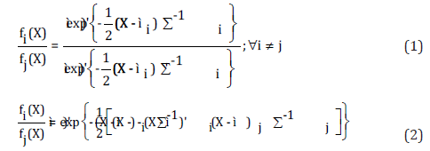
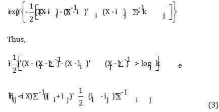
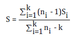 (4)
(4) (5)
(5) (6)
(6) (7)
(7)



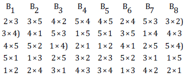
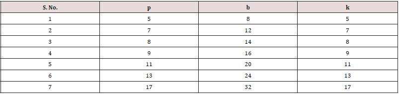
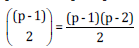 optimal block designs for complete diallel
cross methods (3) with parameters v = p(p-2), b =2(p-2), k =p and
r =2.
optimal block designs for complete diallel
cross methods (3) with parameters v = p(p-2), b =2(p-2), k =p and
r =2.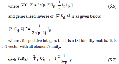
 (5.9)
(5.9)