Lupine Publishers: Lupine Publishers | Optimal Block Design for CDC Method (3)

Lupine Publishers | Current Trends on Biostatistics & Biometrics

Abstract

In the present article, we are presenting the method of construction of block designs for Griffing’s complete diallel cross method (3) by using a complete set of (p-1) mutually orthogonal Latin squares, when p is a prime or a power of prime. The block designs for Griffing’s methods (3) are new and universally optimal in the sense of [1]. The block designs for methods (3) are orthogonally blocked designs. In an orthogonally blocked design, no loss of efficiency on the comparisons of interest is incurred due to blocking. The analysis of data obtained through proposed designs is presented. The analysis includes the analysis of variance, estimation of general combining ability, specific combining ability and reciprocal combining ability. The analysis is illustrated with the help of numerical data. Tables of universally optimal block designs have been provided. AMS classification: 05B15, 62 K 05.

Keywords: Mutually orthogonal latin squares; complete diallel cross; block design; optimality

Introduction

A complete set of (p-1) Latin squares of order p are called mutually orthogonal Latin squares (MOLS), if they are pair-wise orthogonal. MOLS are used for the construction balanced incomplete block designs, square lattice designs and complete diallel cross designs. A set of p-1 MOLS of side p can always be constructed if p is a prime or power of a prime. If p = 4t + 2, t > 1, then there exist more than one mutually orthogonal Latin squares of order p [2]. An exhaustive list of these squares is available. A common experimental design in genetics is the diallel cross, in which pairs of distinct lines (strains) are crossbreed in order to estimate genetic effects. Let p denote the number of lines and it is desired to perform a diallel cross experiment containing v= p(p-1) crosses of the types (i × j) and (j × i) between lines i and j , where i , j = 1,…, p. This type of crossing is the CDC method (3) mating design of [3]. Griffing B (1956) [3] discussed in detail the analysis of CDC method (3) in randomized block design (RBD). Later incomplete block designs were introduced by many authors for diallel cross design [4]. However, this approach did not find favor if one is interested in optimal designs for diallel cross experiments. Several authors such as [5] investigated optimal block designs either for modified diallel i.e. Griffing’s method (4) or for partial diallel crosses to estimate both general and specific combining ability or only general combining ability. .Optimal block designs for CDC method (1) and (2) and variance balanced designs for CDC method (3) in 1- way elimination of heterogeneity set up have been constructed by [6] by using Mutually orthogonal Latin squares(MOLS). The universal optimality and combinatorial aspects for CDC experiment methods (1), (2) and method (4) in the 1-way elimination of heterogeneity setting was studied by many authors. However, optimal block designs for complete diallel cross methods (3) did not received any attention so far in statistical literature. In the present paper, we are proposing block designs for complete diallel cross method (3) through a complete set of (p-1) mutually orthogonal Latin squares, where p is a prime or a power of prime. The rest of this article is organized as follows: in section 2, we give some definitions. In section 3 we give method of construction of block design for method (3) through complete set of MOLS with example. In section 4 we discuss the model and estimation of parameters. In section 5 we discuss optimality in the sense of [1]. In section 6 we discuss about the efficiency factor of this design. In section 7 we give the analysis of CDC method (3) using numerical data.

Some definitions

Definition: A Latin square is said to be in the standard form if the symbols in the first row and the first column are in natural order, and it is said to be in the semi-standard form if the first row are in natural order.

Definition: According to [7], a diallel cross design to be orthogonally blocked if each line occurs in every block r/b time, where r is the constant replication number of the lines and b is the number of blocks in the design.

Method of Construction

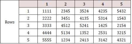
It is known from the work of that when p is a prime or a prime power, it is possible to construct (p-1) MOLS in such a way that they differ only in a cyclical interchange of the rows from 2nd to the path. Here we take a complete set of (p-1) semi - normalized Latin squares for the construction of row-column CDC designs for p varieties because this operation preserves the orthogonally. By superimposition of all the (p-1) semi-normalized orthogonal Latin squares, we obtain a composite square, say, C. Now we transpose the composite C square. The transpose composite square can be partitioned into p rows and p columns where each column contains (p-1) ordered elements in p rows. In the transpose composite square the entry (1, i) contains (p-1) elements i and in the entry (2, i) all the (p-1) elements are different where i = 1, 2, . . p. None of the elements of the entry (2, 1) can coincide with the elements of the entry (1,1). Indeed, if the two elements from this entry are equal to j, then the entry (i,j) contains a pair of element j, which contradicts orthogonality. Hence none of the different elements of the entry (2,1) can coincide with the elements of the entry (1,1) Let us consider that the elements in p rows and p columns represent the number of p varieties. Now we give the method of construction of block designs for [3] methods (3) in two parts by using transpose composite square as follows: Ignoring the first column in the transpose composite square C and perform crosses between any two elements, say, (i × j), in the second column and its corresponding elements in p rows, where i ≠j = 1, 2, . . . p . Thus, we get p cross in the second column. Similarly, we make cross between (j×k) and corresponding elements in other (p-2) columns and p rows, we get mating design for CDC experimental method (3) containing p (p-1) crosses in p (p-1) experimental units. We call this mating design as the first part of CDC experimental method (3). Similarly for second part of CDC design for method (3), we perform crosses between two different elements, say( k × l) other than first selected elements in the second column and corresponding elements in each row and corresponding two elements, say, (r × s) in other cells of the (p-2) columns and corresponding elements in each row, where k ≠l ≠r ≠s = 1, 2, . . . p, we get second part of mating design of CDC experimental method (3) containing p (p-1) crosses in p (p-1) experimental units. Now we juxtaposed the second part with the first part. We get mating design d for CDC method (3) with parameters v = p (p-1), b =2(p-1), k =p and r =2 for CDC method (3). OR Ignoring the first column, we may also get above design by initial row of the design by performing crosses between any two elements, say, (i × j), where i ≠j = 1, 2, . . . p, in first row of the second column and corresponding elements in other (p-1) columns, we get initial row of the design. Now developing the initial row by mod (p), we get mating design as the first part of CDC experimental method (3) in p (p-1) crosses in p (p-1) experimental units. Similarly we may get another initial row by performing crosses between any two different elements other than the first selected elements in the second column and corresponding elements in (p-2) column say, (k × l), where k ≠l = 1, 2, . . . p, we get another initial row. Now developing the second initial row by mod (p), we get mating design as the second part of CDC experimental method (3) of p (p-1) crosses in p (p-1) experimental units. Now we juxtaposed both designs obtained from both initial columns. We get mating design d for CDC method (3) with parameters v = p (p-1), b =2 (p-1), k =p and r =2 for CDC method (3). Example 1. Let us take p = 5, for construction of designs for method (1), we take 4 mutually semi-normalized Latin squares of order 5. After superimposing and transposing, we get the following composite square which has been shown in five rows and five columns. Ignoring first column, we cross any two elements in second column and also cross corresponding elements in other four rows of the second column and similarly we cross corresponding elements in other 3 columns and 5 rows. We get first part of CDC method (1) containing 25 crosses in 25 experimental units. Now we perform crosses between two elements other than the first selected elements in the second column and also corresponding elements in 4 rows of the second column. Similarly, we cross corresponding elements in other 3 columns. We get second part of CDC method (1) containing 25 crosses in 25 experimental units. By juxtaposition both the parts and considering columns as blocks, we get following block design with parameters v = 20, b =8, k =5 and r =2 design for CDC method (3). Block design d For CDC method (3).

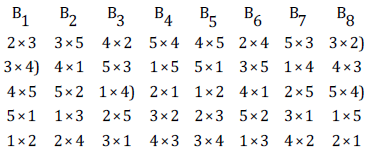
Remark1: According to [7] these designs are orthogonally blocked. In an orthogonal design no loss of efficiency on the comparisons of interest is incurred due to blocking. A block design for which N = θ 1p 1′b is orthogonal for estimating the contrasts among GCA parameters, where N denotes the line versus block incidence matrix and θ is some constant.

Remark2: [8] proved that orthogonally blocked designs remain optimal for the estimation of gca comparisons even in the presence of SCA effects in the model when each cross is replicated twice.

Now we state the following theorem.

Theorem: The existence of a complete set of MOLS of order p, where p is prime or power of prime, implies the existence of optimal block designs for complete diallel cross methods (3) with parameters v = p(p-2), b =2(p-2), k =p and r =2.

Model and Estimation

For the analysis of data obtained from design d, we will follow [5] and [6] two stage procedures for estimating gca, sca effects and reciprocal cross effects with some modification. The first stage is to consider the proposed designs to estimate cross effects, say, ô = (ô 01, ô 02,..., ô (p-1)(p-2) for design d by the following model.

ìy1=+ X ô+ D â + e (5.1)
where y be n×1 vector of observations, 1 is the n×1 vector of ones, X is the n × v design matrix for treatments and D is an n x b design matrix for blocks, that is, the (h,l)th element of X (respectively, of D) is 1 if the hth observation pertains to the lth cross (respectively to lth block),and is zero otherwise, μ is a general mean, τ is a v × 1 vector of treatment parameters, β is a b × 1 vector of block parameters and e is an n × 1 vector of residuals. It is assumed that vector β is fixed and e is normally distributed with E(e) = 0 , V(e) ó= ²I and COV (â, e) = 0, where I is the identity matrix of conformable order. The least square method for the analysis of a proposed design leads to the following reduced normal equations for design d.

ôCd= Q d
Where C_d = r^ä –N k^-ä N´ and Q_d =(Q₁ ,...,Q_v )= T - N k^ä B In the expression above rδ and kδ are diagonal matrices of designs d of order v × p with elements 2 and p in the diagonal respectively. N = X´D is the v × b incidence matrix of the designs d, T = X´ Y is the v × 1 vector of treatment totals and B = D´Y is the b × 1 vector of block totals. The sum of squares due to crosses for design d is Q_d′ C^-_d Q_d with degrees of freedom. = rank (v-1), where is the generalized inverse of with property C C ˉ C = C and expectation and variance of is

ôEa (nQ_d V) = C_d = (Q_d) ó² C_d

Now we will utilize the above equations to estimate the genetic parameters of proposed design. Now we give below the estimation procedure of genetic parameters in Design d.

Estimation of GCA, SCA and reciprocal effects in design d: The second stage is to utilize the fact that the cross effects can be expressed in terms of GCA , SCA and reciprocal effects. Now we can write

ô_ij =g_i +g_j +s_ij +r_ij (5.2)

where gi (gj) is the gca for the ith (jth) parent , sij ( sij = sji ) is the sca for the cross between the ith and the jth parents and rij is the reciprocal effects (rij = -rji) where (i< j = 1,2,…,p) and we also assume that Σ_j s_ij = 0, for all i. The above equation (5.2) can be written in matrix notation as

ô = Z g + s + r (5.3)

where Z = (zui) (u = 1,2, …, v ; i = 1,2, …, p) is the cross and gca relation matrix. zui = 1 if the uth cross has only one parent i. = 0, otherwise Now

C_d ô = C_dZ g + C_d s + C_dr

i.e. E(Q_d) = C_dZg + C_ds + C_dr, óV(Q_d ) = ²C_d (5.4)

Since the matrix is singular, we use the unified theory of least square due to and we get the estimate of general combining ability g.

gˆ = (Z ´C C^-_d Z) ˉ Z´Q_d = (Z´ C_dZ) ˉ ôZ =´C P_d ô 1 (5.5)
where P₁ = (Z´ C_dZ) ˉ Z´ C_d

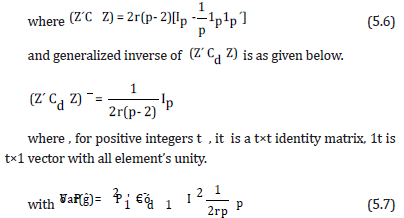
This shows that all elementary contrast among general combining abilities effects through design d is estimated with the same variance. Thus, the design d is variance balanced. We thus have the following result.
Theorem: The design d obtained from super imposition of mutually orthogonal Latin squares of order p, where p is a prime or prime power, is variance –balanced for general combining ability effects.
Now the sum of squares (SS) due to GCA can be calculated as

SS(gca) = Q'_d Z(Z' C_d Z)- Z'Q_d (5.8)
Since estimate of τ does involve reciprocal effects of reciprocal crosses which occur with it in r blocks. To obtain the correct estimate of τ, we eliminate the effects of the reciprocal crosses. So we estimate first the effects of reciprocal crosses. The contrast (τi j – τj i) (i, j = 1, 2,…, p) is estimable and we obtain an estimate of the reciprocal effects of the crosses as given below. Thus we have
rôˆ_ij =-ô_ij ji
Since r_ij =-r_ij , we get ô_ij -ô_ij =2r_ij from equation (5.2), we may write the above expression in matrix notation as

(5.9)

where S = (Su i ) is a v × v matrix with row and column indexed by the pairs (i×j) where i,j = 1,2,…,p, such that If (i×j ,i×j) = (i×j, i×j) then (i×j,i×j) entry of S is 1 and if (i×j,i×j) =( j×i, i×j) then (i×j, i×j) is -1 otherwise 0. Now substituting the estimate of g and r in equation (5.3) and simplifying, we get the estimate of s.

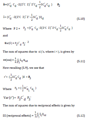
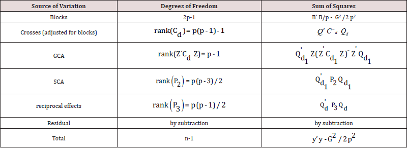
Since P1 1v = P2 1v = P31v = 0 and rank (P1) = p-1 , rank (P2) = p(p-3)/2 and rank(P3) = p(p-1)/2 ,it follows that the ĝ , sˆ and r´ are represented by treatment contrasts that carries (p- 1) and p(p-3)/2 and p(p-1)/2 degrees of freedom respectively. It means the proposed design d allows for general combining ability, specific combining abilities and reciprocal effects to be estimated independently.

The ANOVA is then given in Table 1.

Table 1.

Lupinepublishers-openaccess-Biostatistics-Biometrics-journal

Optimality

Now we take up the optimality aspects. The optimality criterion chosen is the minimization of the average variance of the best linear unbiased estimators of all elementary comparison between general combining ability effects. According to [1], a design is universally optimal in a relevant class of competing designs if:
a. The information matrix C of the design is completely symmetric means C has all its diagonal elements equal and all its off – diagonal elements equal; and
b. The matrix C has maximal trace over all designs in the class of competing designs.
c. Now using proposition of [1], we have the following theorem.
d. Theorem 3: Let d* ɛ D (p, b, k) be a block design for diallel cross, satisfying
e. trace (Cd*) = k-1b{2k(k-1-2x) + p x (x+1)} and
f. Cd* = (p-1) -1 k--1 b {2 k (k -1-2x) + p x (x+1)} (Ip – p-1 1p 1′p) is completely symmetric.
where x = [2k/p], and for square matrix A, tr(A) stands for the trace. Ip is an identity matrix of order p and 1p 1′p is a p × p matrix of all ones. Furthermore, using d* ε D (p, b, k) all elementary contrasts among gca effects are estimated with variance

Then d* is universally optimal in D (p, b, k) and in particular minimizes the average variance of the best linear unbiased estimators of all elementary contrasts among the general combining ability effects.

In our case the C matrix of designs d is (Z´ C_d Z) which is completely symmetric. From (5.6) it is easy to see that the trace of design d is 2 r p (p-1) which is equal to Theorem 3. Hence, we have the following theorem.

Theorem: The designs d obtained from mutually orthogonal Latin squares of semi standard order after superimposing (p-1) mutually orthogonal Latin squares for diallel crossing experiments method (3), are universally optimal.

Illustration

We show the essential steps of analysis of a diallel cross experiment, using an incomplete block design proposed in this paper. For this purpose, we take data from an experiment on the number of tillers per plant in pearl millet, reported by on page 180. The author used a randomized complete block design with v =20 as he considered all possible p (p-1) crosses including selfing and reciprocal crosses, among p =6 inbred lines. On the purpose of illustration, we take the data of relevant crosses from this experiment. The design chosen is d. There are 20 crosses and the design have 8 blocks, each of size five. Each cross is replicated twice. The layout and observations in parentheses are given below.

The following are the vector of treatment total, block total and adjusted treatment total respectively.
The following are the vector of treatment total, block total and adjusted treatment total respectively.
T = ( 12,14,13,15,7,10,5,10,18,18,22,16,16,7,10,8,11,19,18,15, 26)
B = (33, 30, 32, 36, 35, 30, 34, 38)
Q= ( -1.6, 2.0, -0.2,0.2, -7.8, -3.6, -7.0, -3.2, 4.8, 3.2, 2.4, 4.0, -5.0, -3.2, -6.8, -2.6, 5.4, 6.0, 1.8, 11.2) A NOVA and estimates of GCA, SCA and reciprocal effects along with their standard errors are shown in [Tables 4-7].

Table 2: Analysis of variance of proposed design d as mating and environment design.