Abstract
Although the well-known standard Lagrange multiplier method (LMM) can
even produce higher accuracy and easier implementation than other
conventional schemes (e.g., the modified variational principle, the
Nitsche's method), however it inherently owns many difficulties in
solving the system of discretized equations, mainly caused by new
unknown Lagrange multipliers. The LMM naturally increases the problem
size and leads to a poorly conditioned matrix equation. The singularity
is also often encountered because of inappropriate selection of
interpolation space for the Lagrange multiplier. In this paper, we
propose an improved method, called reduced Lagrange multiplier method,
which can overcome such drawbacks raised by the LMM in treating the
Dirichlet-type boundary conditions in terms of Isogeometric Analysis. By
simply splitting the system equations into boundaries and interior
groups, the size of system equations derived from the LMM is reduced; no
additional unknowns have been added into the resulting system of
equations; the Lagrange multiplier is hence disappeared; and more
importantly the singular problem mentioned is avoided. The accuracy and
convergence rates of the proposed method are studied through three
numerical examples, exhibiting all the desirable features of the method.
Optimal convergence rate and high accuracy for the present method is
found.
Keywords: NURBS; Isogeometric analysis; Dirichlet boundary conditions; Lagrange multiplier method; Finite element method
Abbrevations: LMM: Lagrange Multiplier
Method; IGA: Iso-Geometric Analysis; CAD: Computer-Aided DBCs: Design
Boundary Conditions; DM: Direct Method; LSCM: Least-Squares Collocation
Method; RLMM: Reduced Lagrange Multiplier Method
Introduction
The Isogeometric analysis (IGA) [1] employs the same computer- aided
design (CAD) spline basis functions (e.g., NURBS, T-splines) to describe
exact geometries and approximate physical responses. The IGA offers
possibilities of integrating finite element analysis into CAD design
tools and avoids mesh generation process and subsequent communication
with a CAD model during refinement. The IGA has shown to be a highly
accurate and robust approach for numerical simulation with exact
geometry representation even with coarse mesh [2]. Moreover, the
high-order smoothness of the NURBS basis functions allows for a direct
construction of rotation- free plate/shell formulations [3,4] and is
attractive for solving PDEs that incorporate fourth-order (or higher)
derivatives of the field variable, such as the Hill-Cahnard equation
[Gomez et al., 2008] [5] and gradient damage models [6].
The IGA has shown to be an effective approach in solving engineering
problems as a large number of works on the theory and application of IGA
have been conducted and reported in literature, including mathematical
properties [7,8], integration method [9,10], spline techniques [11],
fluid mechanics [12], fluid- structure interaction [13], plate/shell
structures [14-17], electromechanic [18], magneto-electro elastic [19],
shape optimization [20], fracture mechanics [21], and unsaturated flow
problem [22]. Despite the efforts dedicated to the IGA in recent years
and the significant progress has been made, some relevant technical
aspects still require further studies; and among others the imposition
of the Dirichlet-type essential boundary conditions (DBCs) in the IGA is
an important technical issue. Given the non-interpolating nature of the
NURBS basis, similar to moving least-squares [23], the properties of
Kronecker delta are not satisfied, directly imposing DBCs is difficult,
and special techniques are hence required.
Hughes et al. [1] addressed a direct method (DM) for DBCs enforcement
to the control points. However, Wang & Xuan [24] found that the DM
may induce significant errors with deteriorated convergence rates, and a
special DBC treatment technique in terms of mesh less computation for
contact problems [25] is presented, which is accomplished by separating
the interior and boundary points on the basis of the mixed
transformation method. They numerically illustrated that the improved
approach produces favorable solution accuracy and optimal convergence
rates compared with DM. However, the selection of boundary interpolation
points should be emphasized in order to avoid a singular transformation
matrix. Koo et al. [26] recently extended this method to iso geometric
shape design.
Costantini et al. [27] applied the quasi-interpolation method to set
inhomogeneous DBCs in the IGA on the basis of generalized B-splines to
eliminate the solution of large global linear systems. Lu et al. [28]
presented a technique to blend NURBS with Lagrangian interpolation in
the essential boundary and allow the direct imposition of prescribed
values. Other strategies based on a modified weak-form equation, such as
Nitsche's method [29] and Lagrange multiplier method (LMM) have been
adopted in NURBS-based IGA. Recently, De Luycker et al. [30] proposed a
least- squares collocation method (LSCM) for imposing arbitrary DBCs in
extended IGA. Govindjee et al. [31] later improved the LSCM by offering
an efficient local least-squares algorithm to global least squares.
However, LSCM is affected by the number of interpolating points. Thus,
an important issue on how to choose the location and number of
interpolating points precisely arises. The LMM is widely used in
weak-form methods for DBCs enforcement [32].
The LMM offers solutions higher accuracy than the modified
variational principle [33]. The implementation of LMM is simpler and
more straightforward than the Nitsche's method [32]. However, the LMM
introduces a new unknown Lagrange multiplier, which makes it difficult
in selection of interpolation space for the Lagrange multiplier so that
singular issues in solving the system of equations are avoided. In this
paper, we present a new improved method, reduced Lagrange multiplier
method (RLMM) for effective treatment of the DBCs in terms of IGA. Given
that the NURBS control points can be clearly partitioned into boundary
and interior groups and that the NURBS basis functions of interior
control points vanish at the boundary [24], we divide the system
equation of the LMM into boundary and interior groups.
Thus, the size of the equation system is now reduced and the
shortcomings of the LMM can hence be overcome. Furthermore, the choice
of the interpolation space for the Lagrange multiplier is studied
numerically and is discussed in numerical results. The rest of this
paper is organized as follows. Section 2 presents a brief on the
NURBS-based IGA. Section 3 details the RLMM for essential boundary
condition treatments in IGA. Numerical examples are considered in
Section 4 to verify the accuracy and effectiveness of the present
method. The conclusions are drawn in Section 5.
NURBS-Based Isogeometric Analysis
NURBS basis functions
In a 1D parametric space ξε[0,1], a knot vector κ(ξ) to construct the B-spline basis functions is a set of non-decreasing numbers written as  where and are the number of basic functions and the order of basic
functions, respectively. Given a knot vector κ (ξ), the B-spline basis
function of degree p, written as Ni,p (ξ), is defined recursively as follows [34]
where and are the number of basic functions and the order of basic
functions, respectively. Given a knot vector κ (ξ), the B-spline basis
function of degree p, written as Ni,p (ξ), is defined recursively as follows [34] 
and

The NURBS basis function Ri,p (ξ) in the framework of partition of unity is constructed by a weighted average of the B-spline basis functions [35]:
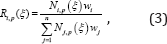
where is the ith weight.
Similarly, the bivariate NURBS basis functions are expressed in the following form:

Where represents the 2D weight; Ni,p (ξ) and Nj,q
(η) are the B-sp line basis functions defined on knot vectors κ(ξ) and
κ(η) , respectively, following the recursive formula shown in Eqs. (1)
and (2).
The NURBS basis functions are non-interpolatory in the interior
parametric space interval. Therefore, essential boundary conditions
cannot be applied simply by enforcing individual values to the control
points.
By using the NURBS basis functions, a NURBS surface of order in the
direction and order in the direction can be constructed as follows:

where Pij are the coordinates of the control points in two dimensions.
Governing equations and discretization
Without loss of generality, we consider a 2D isotropic elastic
problem whose problem domain is with a boundary ( and ), the
corresponding governing equations are expressed as follows:
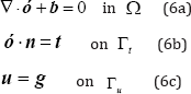
where ∇ denotes the gradient operators; ó is stress tensor; b and t are the body and surface force vectors, respectively; n is the normal vector on Neumann boundary Γt ;g is the known displacement on Γu .
The total potential energy of the system can be constructed as follows:

In the NURBS-based IGA, an isoparametric concept is adopted and
the NURBS basis functions are used for geometric modeling and analysis:
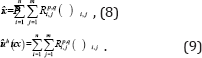
After the control points are rearranged with a unified subscript , the field approximation can then be written as follows:

where Î is the parametric coordinate; RI (Î) denotes the NURBS basis function at control point I ; NP is the total number of control points.
On the basis of the principle of minimum potential energy and by
substituting the approximated displacements of Eq. (10) into Eq. (7), a
system of discretized algebraic equations can be obtained as follows:
KU = f , (11)
where is the vector of the unknown variable at control points; and
are the global stiffness matrix and external force vector at control
points, respectively.
The element contributions to and are as follows:
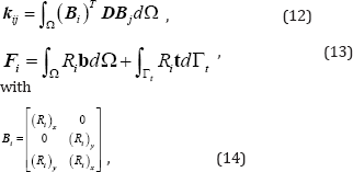
where D is the Hooke's elasticity matrix.
Reduced Lagrange Multiplier Method For Dirichlet Boundary Conditions
The NURBS basis functions that are often used in the IGA do not
satisfy the Kronecker delta function, and the direct imposition of uI (x) = gI (x)
on the control points may induce significant errors with deteriorated
convergence rates [12]. The novel RLMM is presented in the following.
Reduced lagrange multiplier method
The LMM is easy to understand and implement because it has been
widely used for the enforcement of DBCs. However, the LMM increases the
problem size and leads to a poorly conditioned matrix equation. To
overcome these shortcomings, we modify the standard LMM such that the
size of the equation system is reduced. We named the modified method the
RLMM. By applying the LMM, the constrained weak form is obtained as
follows:

The matrix form of the LMM is derived as follows [Ghorashi et al., 2012]:

The Lagrange multiplier is approximated by the NURBS basis functions as follows:

The degrees of freedom (DOF) u for the control points discretized in the structure can be categorized into two groups: the constrained DOF uB that is the collection of control points ( ) for boundary description, and the unconstrained DOF uA
that is the collection of control points ( ) for interior domain
description. The NURBS control points can be clearly partitioned into
boundary and interior groups because the corresponding NURBS basis
functions associated with the interior control points vanish at the
boundary. Thus, field approximation can be partitioned as follows:
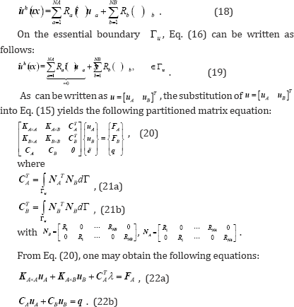
Given that the basis functions of interior control points ( NA) vanish identically at the boundary Γu ,CA =0, Eqs. (22a) and (22b) can then be respectively written as follows:
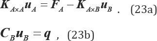
The results systems Eqs. (23a) and (23b) show that the additional
unknowns, the Lagrange multiplier are disappeared, the singular problem
can be avoid and the size of the equation system is actually reduced to
an (n-NB) × (n-NB) matrix problem. Besides, as the NURBS basis functions
are used as the interpolating functions of finite element analysis and
the Lagrange multiplier (Eq.(17)), so the coefficients 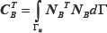 is similar to a 1D mass matrix along the boundary, and the full
quadrature (the number of Gauss points in each direction is p+1) is used
to sure that it has an inverse.
is similar to a 1D mass matrix along the boundary, and the full
quadrature (the number of Gauss points in each direction is p+1) is used
to sure that it has an inverse.
Further discussions to the method
Several possibilities are available for the choice of the
interpolation space for the Lagrange multiplier, such as (1) the
Lagrange shape functions or (2) the same shape functions used in the
interpolation of U (i.e., the NURBS basis functions in the IGA).
To verify the Babuska-Brezzi stability condition and impose accurate
essential boundary conditions, choosing the interpolation of the
Lagrange multiplier is important. In the IGA, the matrix form of the LMM
equation is expressed as follows:
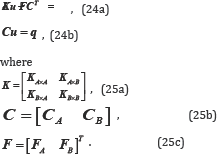
The combination of Eqs. (24a) and (24b) perform a block-wise Gaussian
elimination to obtain the pressure Schur complement as follows:

The question now is whether CK-1CT is invertible. K-1 is usually invertible for Laplace- and Poisson-type problems; therefore, we only need to consider whether CCT can be invertible. The Babuska-Brezzi stability condition also ensures CCT to be invertible. In the IGA, CA= 0; thus, CCT is reformed to becBcTB . If the NURBS basis functions are used as the interpolating functions of the Lagrange multiplier (Eq.(17)), then  is similar to a 1D mass matrix, and CBCTB
can be invertible. Therefore, the NURBS basis function is a stable
space for the Lagrange multiplier to impose essential boundary
conditions in the IGA. The NURBS basis function can obtain an acceptable
solution on the numerical examples (Section 4), and the resulting
system of equations will not be singular even if the number of Lagrange
multipliers is large.
is similar to a 1D mass matrix, and CBCTB
can be invertible. Therefore, the NURBS basis function is a stable
space for the Lagrange multiplier to impose essential boundary
conditions in the IGA. The NURBS basis function can obtain an acceptable
solution on the numerical examples (Section 4), and the resulting
system of equations will not be singular even if the number of Lagrange
multipliers is large.
Numerical Examples and Discussion
In this section, three 2D examples are considered to show the
accuracy and performance of the RLMM approach. The number of Gauss
points in each direction is p+1 in all studies, with p being the order
of the NURBS basis function. For convergence analysis, the h-refinement
strategy is applied and knots are added to the middle of the knot spans.
Moreover, three different measurements of error are calculated to
assess the accuracy of the present method. The L2 error norm is
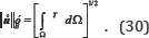
expressed as follows:

where and are the exact and approximate displacements, respectively.
The H1 error norm is expressed as follows:

The strain energy error norm is expressed as follows:

where and are the exact and approximate strains, respectively; and are the exact and approximate stresses, respectively.
The exact strain energy norm is defined as follows:
Laplace problem on a square domain
The first example considers the Laplace problem. The governing equation and the boundary conditions are expressed as follows:
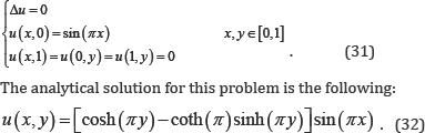
Figure 1: Initial geometry: physical mesh (a) and control mesh (b).
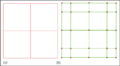
As shown in Figure 1, the initial geometry is constructed by a NURBS
surface of order p = 3 for both directions with unit weights. The
initial parameter space is given by knot vectors κξ = {0,0,0,0,0.5,1,1,1,1} and κη =
{0,0 ,0,0,0.5 ,1,1,1,1} . For the convergence analysis, h-refinement is
used to refine the mesh by knot insertion. The refined meshes have 16,
64, 256, and 1024 elements (Figure 1).
The convergence results of the RLMM, LMM and the DM are shown in
Figs. 2 and 3, respectively. The optimal convergence rates are obtained
for the present method and LMM while the results based on the RLMM are
identical to those from the LMM. A quadratic convergence rate in the L2
error norm and a cubic convergence rate in the H1 error norm are
obtained that are comparable with the quadratic convergence rate in both
cases for the direct imposition of boundary conditions. We can also
predict that the RLMM can compute faster than traditional LMM because
only an (n-NB)x(n- NB) matrix problem (Eq.23) needs to be solved in the
former rather than an ill-conditioned (n+NB)x(n+NB) matrix problem [Eq.
(16)] in the latter.
Table 1: Comparison of the DOFs and condition number used for the computation among different methods.

The comparison of different methods on the number of degrees of
freedom and matrix condition number are presented in Table 1. Divided
the total DOF n into boundary DOF NB and interior DOF NA, it can be seen
from Eq.(23) that the RLMM owns the same number of DOF as the DM, but
the boundary DOF NB is imposed directly in DM while it obtained by
solving the system of equation with smaller size Eq. (23a) in the RLMM.
The total number of unknowns in the LMM will be n+NB as Lagrange
multiplier unknowns are equal to boundary DOF NB. On the other hand, the
matrix condition number of RLMM and DM are the same as shown in Eq.
(23b). As shown in Table 1, the matrix condition number of LMM is three
orders of magnitude larger than the RLMM and DM which is even worse for
complicated problems. In conclusion, the RLMM has the same matrix
condition number as the DM but needs to solve an Eq. (23a) to get the
boundary unknowns NB. Compared with Eq. (23b), Eq. (23a) is smaller and
would not waste too much time. However, compared with the DM and LMM,
additional unknowns and bad matrix condition number are found for the
LMM.
Figure 2: Comparison of L2 error norms for Laplace problem on a square domain.
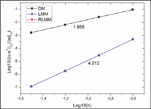
The RLMM yields the same accuracy as the LMM while avoiding bad
matrix condition number as the DM and also the singularity often met in
the LMM for large number of degrees of freedom is no longer encountered
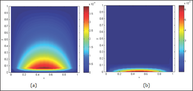
(Figures 2 & 3). The absolute error  distributions utilizing 256 elements are depicted in Fig. 4 to show the
accuracy of the proposed approach. The following can be observed from
the results: (1) the error domain derived from the RLMM is small,
whereas less accuracy at the boundary can be found for the DM; (2)
according to the error distributions, although the maximum value of
error given by the DM is smaller than that by RLMM, the error region of
DM is larger than the those of RLMM (Table 1) (Figure 4).
distributions utilizing 256 elements are depicted in Fig. 4 to show the
accuracy of the proposed approach. The following can be observed from
the results: (1) the error domain derived from the RLMM is small,
whereas less accuracy at the boundary can be found for the DM; (2)
according to the error distributions, although the maximum value of
error given by the DM is smaller than that by RLMM, the error region of
DM is larger than the those of RLMM (Table 1) (Figure 4).
Figure 3: Comparison of H1 error norms for Laplace problem on a square domain.
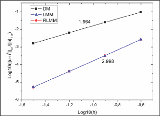
Figure 4: Distributions of absolute errors obtained by (a) DM, (b) RLMM.
A Cantilever beam
A cantilever beam with length L = 48 units and height H = 12 units
subjected to a parabolic traction at the free end as shown in Fig. 5 is
considered. The material properties of the beam are taken as follows:
Young's modulus E = 3.0x10⁷ units, Poisson’s ratio v = 0.3. Plane stress
conditions are assumed. The imposed parabolic traction is expressed by
the following:
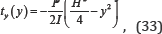
where I = H3 /12 denotes the moment of inertia,
the shear force applied is P = 1000 units, and the left edge of the
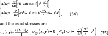
beam is clamped. The analytical displacements of this problem are given
by the following [35,36]:
The order of the NURBS basis functions is p = 2 and the initial parametric space is defined by knot vectors . κξ=κη,={0’0’0’0.5’U’1}
The weights associated with all the basic functions are set to one;
thus, the NURBS basis functions are identical to the corresponding
B-spline functions. The meshes used for the convergence study are 4 x 4,
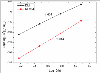
8 x 8, 16 x 16, and 32 x 32 elements. The results of the L2 and strain
energy error norms shown in Figs. 6 and 7 clearly confirm that the
proposed method has smaller solution errors than the DM and preserve the
optimal convergence rates (L2 error norm: 3.016, H1 error norm: 2.014)
(Figure 5-7).
Figure 5: Description of cantilever beam problem.
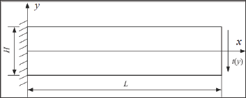
Figure 6: Comparison of L2 error norms for cantilever beam problem.

Figure 7: Comparison of strain energy error norms for cantilever beam problem.
Infinite plate with a circular hole
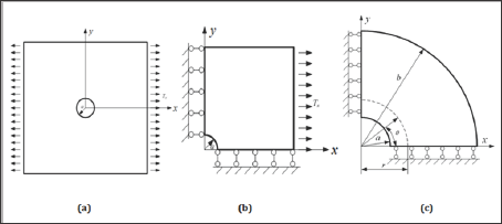
The last example deals with a plane stress infinite plate with a
central circular hole under the x-direction traction Tk =1 unit (Figure
8a). Owing to geometrical symmetry, a quarter of the domain is simulated
(Figure 8b). To avoid the singularity in the geometric representation,
we further consider a finite annular plate in the numerical model
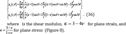
(Figure 8c). The exact displacements using Eq. (36) are imposed on the
inner and outer edges of the annular plate. The analytical displacement
solutions are expressed as follows [35]:
Figure 8: Schematic description of (a) an infinite
plate with a circular hole, (b) a quarter of the geometry, and (c) a
finite annual plate used for numerical implementation model.
The geometry and material parameters are the radius of the
circular hole a = 1 unit, the outer radius b = 4 units, Young's modulus E
= 105 units, and Poisson's ratio v = 0.3. The initial geometry for this
problem is shown in Figure 9. The refined meshes used in the
convergence analysis are 4 x 4, 8 x 8, 16 x 16, and 32 x 32 elements.
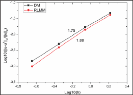
The results of L2 and the strain energy error norms are analyzed and
respectively plotted in Figures 10 & 11. The proposed method has
less solution errors and achieves optimal convergence rates, thus
outperforming DM (Figure 9-11).
Figure 9: Initial geometry of (a) physical mesh and (b) control mesh.
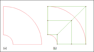
Figure 10: Comparison of L2 error norms for infinite plate with a circular hole.
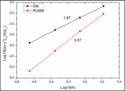
Figure 11: Comparison of strain energy error norms for infinite plate with a circular hole.
Conclusion
The Dirichlet boundary conditions (DBCs) in IGA are studied by
developing an accurate treatment method, the RLMM, for overcoming the
difficulties in the enforcement of DBCs. Compared with the standard LMM,
the size of equation system is reduced as the resulting system of
equations have made no additional unknowns, the Lagrange multipliers are
thus disappeared and the singular problem in LMM is avoided. The
benefit of the proposed approach can gain even greater if the number of
degrees of freedom of the discretization system is relatively large. The
choice of the interpolation space for the Lagrange multiplier is
addressed in detail. As a result, the NURBS basis function is found to
be a stable space for the Lagrange multiplier for which the DBCs in the
IGA is imposed.
Nevertheless, the realization of the improved method in the treatment
of DBCs in the IGA is straightforward, and can be integrated into
existing IGA codes with less effort. Thus, the improved method can be
ideal candidate for practical problems. Based on the numerical
investigation of the convergences, the new method yields high accuracy
on the solutions and optimal convergence rates, confirming the
effectiveness of the enhanced treatment technique of the DBCs in the
IGA. The level of accuracy and convergence rates achieved by the RLMM is
better than the DM.
Acknowledgment
This work was supported by Natural Science Foundation of Hunan
Province of China (2017JJ3306), Foundation of the Education Department
of Hunan Province of China (17C1532), and Research Foundation of
Xiangtan University (16QDZ15). The financial supports are gratefully
acknowledged.
Read More Lupine Publishers Trends in Civil Engineering and its Architecture (TCEIA) Please Click on Below Link: https://lupinepublishers-civilengineering.blogspot.com/