Showing posts with label Journal of Civil Engineering Research. Show all posts

Monday, 9 May 2022

Lupine Publishers| Estimating Deformations of Laboratory Structures Subjected to Loadings Using Images Collected with Phone Camerase

 Lupine Publishers| Journal of Civil Engineering and its Architecture


Introduction

A Fundamental civil engineering knowledge is the ability to understand, explain and calculate deformations of/in civil structures. New civil engineers acquire this knowledge at universities in material science, engineering mechanics and introduction to structural engineering modules. Structural deformations can be calculated when knowing material properties, geometry and boundary conditions of a structure and loads that are applied on/to it. Inverse engineering can be employed if deformations of a structure are known, but some other parameters are not known. Theoretical formulae are then tested using laboratory test beds, usually beams. Laboratory technicians are responsible for the acquisition of deformation measurements of laboratory tests. Their time is often limited and so is the number of available measurement collection devices such as dial gauges and strain gauges. If devices that do not log measured deformations are employed, information of structural deformations or response might be lost or readings might not be collected at required intervals. However, all laboratories do not offer luxury of sensors that are available at hand and technicians, which would have time to install sensorsand collect data when needed, especially if this as to be done with a short period of notice. This paper introduces a low-cost vision-based system for deformation estimations of laboratory structures.

Significant research is done in the image processing and photogrammetry fields, which is reviewed in recently published paper [1]. Ho et al. [2] demonstrated that two camcorders when used simultaneously can capture displacements of civil structures. Ye at el. [3] employed high-resolution industrial digital cameras with extended-range zoom lenses to collect dynamic movements of long- span bridges and derived structural displacements from collected images. In above examples, camcorders or high-resolution cameras were employed. This study shows that mobile phone cameras can be used to do the above. DefoMonit- software introduced in this paper and developed at Nottingham Trent University (NTU) [4], can analyse consecutively collected images of structures subjected to loadings and estimate structural deformations. DefoMonit, in contrast to proprietary software, is free for students and academics. The next sections provide general introduction to the vision-based system and a laboratory case study.

Methodology

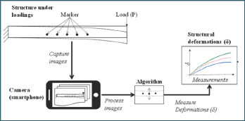
Figure 1: A schematic representation of condition assessment of a structure under loadings using a low cost vision-based measurement collection system with a smart phone camera.

Lupinepublishers-openaccess-journals-Civil-engineering-Architechture

Figure 1 presents a proposed system for estimating deformations such as deflections in laboratory test-beds. A selected test-bed is a cantilever beam subjected to loadings. Markers or points of interest are drawn on the surface of the beam. Images are captured with a phone camera while the load is applied to the beam. When analysing collected images with DeforMonit, the location of the markers is tracked, and structural deformations are estimated.

A laboratory structure subjected to loadings

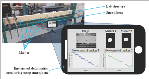
Figure 2: Envisioned set-up of the vision-based system using a phone to collect and DeforMonit to analyse images for deformation estimation of a cantilever at the lab in (NTU).a.

Lupinepublishers-openaccess-journals-Civil-engineering-Architechture

An illustration of the proposed system using a phone for deformation monitoring of a cantilever beam is shown (see Figure 2). Markers are drawn on the face of the beam. A phone is placed at a preferred distance from the laboratory structure. Setting the correct distance, at which images are taken, has a direct impact on the resolution of images and calculated structural deformations. Understanding of structures is required to provisionally estimate expected movement of the laboratory structure. The collected images are analysed using DeforMonit, and time series of estimated deformations are generated.

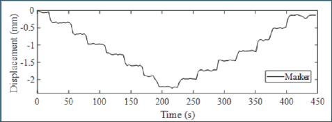
Figure 3: Time series of vertical movements of a selected marker on the timber beam.

Lupinepublishers-openaccess-journals-Civil-engineering-Architechture

Consider the timber cantilever shown in Figure 2. The cantilever is 900mm long, 45mm wide and 70mm deep. A load is applied manually at its right end using 5N load step. When the applied load reaches 35N, it is removed using 5N steps. Samsung A3 phone is deployed to capture images of the cantilever under loadings. The phone is placed 800mm away from the cantilever capturing its entire length. The movement of a marker at its far right end is tracked and plotted in Figure 3.

Summary and Conclusion

   This synopsis introduces DefoMonit, a freeware for image analyses of structures subjected to loadings for accurate estimations of structural deformations. The accuracy of estimated deformations using DeforMonit is validated on laboratory and full-scale structures [4]. Students at NTU use DeforMonit in their final year project. In this paper, an example showing deformations of a cantilever beam subjected to manually applied loads is demonstrated in Figure 3.

Read More About Lupine Publishers Journal of Civil Engineering and its Architecture Please Click on Below Link: https://lupinepublishers-civilengineering.blogspot.com/

Monday, 24 January 2022

Lupine Publishers| Trends in Developing Critical Elastic Buckling Formula for Fixed Rectangular Plate Subjected To a Concentrated Load

 Lupine Publishers| Journal of Civil Engineering and its Architecture


Abstract

   Lateral buckling analysis of fixed rectangular plates under the lateral concentrated load is an interesting problem. However, there is not a determined equation to calculate the critical elastic buckling strength of such plate. This paper presents the equations of the previous studies by Cheng and Yuan and analyzes the critical buckling strength of the plate calculated by finite element method (FEM). Finally, discussion and suggestion on the trends in developing critical elastic buckling formula for such plate are made.

Short Communication

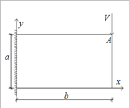
Rayleigh-Ritz method is commonly used energy method to calculate the elastic buckling strength of a plate Qu [1]. The total potential energy of a structure is π = U + W , where U is the buckling deformation potential energy and W is the external potential energy. The critical buckling strength of a structure can be calculated once . For an end-fixed rectangular plate subjected to a concentrated load, the mechanical diagram is shown in (Figure 1). The buckling deformation potential energy of the plate can be determined as:

Figure 1: Mechanical diagram of the plate.

Lupinepublishers-openaccess-journals-Civil-engineering-Architechture

Lupinepublishers-openaccess-journals-Civil-engineering-Architechture

Where D = Et3 /12(1 -μ2) is the buckling stiffness of the plate; E and t is the elastic modulus and the thickness of the plate, respectively; n is Poisson's ratio of the material used for the plate. ρ is the buckling deformation function, and ωxx,ωxy,ωyy are the partial derivatives of the buckling deformation function.

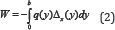
The external potential energy of the plate can be calculated by:

Lupinepublishers-openaccess-journals-Civil-engineering-Architechture

Where q is the lateral concentrated load and Δx (y) is the out- of-plane displacement of the plate caused by the buckling of the plate. It can be found that the critical buckling strength of the plate is determined by buckling deformation function. Therefore, it is important to assume a feasible buckling deformation function for the analyzing plate. Cheng [2,3] proposed the buckling deformation function as:

Lupinepublishers-openaccess-journals-Civil-engineering-Architechture

Yuan [4] modified the buckling deformation function of Cheng (1988), and given it as:

Lupinepublishers-openaccess-journals-Civil-engineering-Architechture

Where f1 and f2 are unknown variables to describe the various types of the buckling deformation function, thus the critical one could be found in these functions. Through case studies conducted by Yuan [4], the critical results calculated by Eq. (4) were lower than the results calculated by Eq. (3). Thus it was concluded by Yuan [4] that the Eq. (4) was more accurate for determining the critical buckling strength of the plate. However, Yuan [4] proposed another buckling deformation function as:

Lupinepublishers-openaccess-journals-Civil-engineering-Architechture

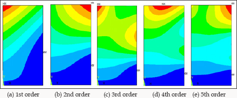
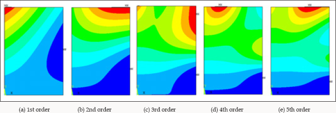
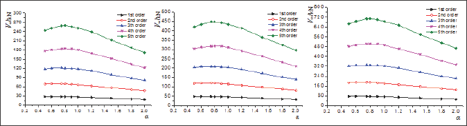
With developing of the computer-aided calculating method such as finite element method (FEM), the buckling modes of the analyzed plate can be depicted more visually. In this paper, the FEM model for the analyzed plate is generated by the FEM software ANSYS 12.0. A target plate is selected with a constant value of 2.7 m in height, and the elastic modulus of the plate is 206 GPa. The width of the plate is changing from 1.35 m to 3.6 m, and three cases with height-to-width ratio 2.0, 1.5 and 0.75 are analyzed. The thickness of the plate is 10 mm, 12 mm and 14 mm. Eigen value buckling analysis of these FEM models is conducted by Block Lanczos method. The first 5 orders of the buckling modes of these plates are generated, and the cases of α=2.0, α=1.5 and α=0.75 with 10 mm in thickness are depicted from (Figures 2-4). The critical strength of these plates for which calculated by FEM are shown in (Figure 5).

Figure 2: Buckling mode of the plate with ɑ=2.0.

Lupinepublishers-openaccess-journals-Civil-engineering-Architechture

Figure 3: Buckling mode of the plate with ɑ=1.5.

Lupinepublishers-openaccess-journals-Civil-engineering-Architechture

Figure 4: Buckling mode of the plate with ɑ=0.75 and t=10 mm.

Lupinepublishers-openaccess-journals-Civil-engineering-Architechture

Figure 5: Relationship between the critical strength and of and the � Jiang et al. [3].

Lupinepublishers-openaccess-journals-Civil-engineering-Architechture

Discussion and Suggestion

As shown in (Figures 2-4), it can be found that the consequence of the buckling modes is moved by changing the height-to-width ratio of the plate. High-order buckling mode may be occurred in the plate with lower height-to-width ratio. According to the studies conducted by Cheng and Yuan, only two variables were in their equations, and the cosine function and polynomial function were used to describe the buckling modes of the analyzed plates. However, two variables might not be used to present the high-order buckling mode of half-waves more than three. Such functions limit more degree of freedom (DOF) of the plate, and the critical buckling strength calculated from such functions is larger than the correct value.

Thus this paper suggests the buckling deformation function as follow:

Lupinepublishers-openaccess-journals-Civil-engineering-Architechture

Such function should be following the boundary conditions of the plate, and they are:

Lupinepublishers-openaccess-journals-Civil-engineering-Architechture

The Eq. (6) combines the double series function derived by Navy, and the single series function derived by Levy, and aims to find the most proximal buckling deformation function for the critical buckling mode of such plate.

Read More About Lupine Publishers Journal of Civil Engineering and its Architecture Please Click on Below Link: https://lupinepublishers-civilengineering.blogspot.com/


Tuesday, 2 November 2021

Lupine Publishers| Experimental Investigation on FRP Composite Compression Members

 Lupine Publishers| Journal of Civil Engineering and its Architecture


Introduction

   In the last 25 years, fiber-reinforced polymer (FRP) composite materials have been considered to be used in various civil engineering applications such as the cooling tower system, waste water treatment plant, pedestrian bridges, reinforced concrete rebars, structure strengthening members, and some metallic sensitive specialized buildings. This review of study is only concentrated on the experimental investigation of GFRP composite compression members made from glass-fiber and polyester-based and vinylester-based polymers in a pultrusion process.

Experimental Program

The experimental program includes 300+GFRP composite compression members with various dimensions, length, and crosssection configurations. Two sections have closed configurations; square box and round sections, three sections have open configurations; wide-flange, angle and I-sections. The length varies from 0.33m to 7m, the wall thickness of each members varies from 3mm to 10mm. The compression members were tested in the lab with 3-5 specimens for each group. The objectives of the research are to determine the allowable compressive stress, ultimate load, the effective length, and mode of failure.

Analysis and Discussion

    i. From the material point of view, the GFRP composite materials can be applied to civil engineering structures as long/short columns, and as structural bracing elements. Particularly in an adverse environmental conditions, because of the corrosion resistance nature of the material. The bearing capacity of the compression member can be improved if the material constituents are replaced by the higher quality of fiber such as carbon fibers and aramid fibers, and an advanced polymers such as epoxies, but the material cost for construction will also be increased.

    ii. The ultimate load capacity and the mode of failure for GFRP composite compression members depend on the length and the cross-section configuration of the member. For a given length and section shape, the significant parameters are the slenderness ratio and the flange-width to thickness ratio.

    iii. The Euler's curve established from the test shown the dividing line for long and short membersbased on slenderness ratio (kl/r). For various configurations the values of kl/r are presented as follows (Table).

Table 1

Lupinepublishers-openaccess-journals-Civil-engineering-Architechture

iv. In general, the bearing strength of GFRP is about 200Mpa.

For closed section, the square box and round tube sections have shown bearing failure for short members and buckling failure for long members. For open section, the wide-flange, angle and I-sections have indicated bearing and/or local buckling failure mode for short and local/global bucking mode of failure for long compression members.

 v. Compression members with I-sections have shown a sudden failure by global buckling at no warning in any fashion. It is recommended that the application of I-section compression members needs to be cautious (Figure).

vi. One of the interesting observation is that, the moment before failure, particularly for long compression members, a light color appears and reflected on the surface under the illumination of the lab. This phenomenon may be attributed to the stress level changes or high stress concentration at the position of failure. A photo-elasticity approach analysis may be interested in looking into the results. 

Read More About Lupine Publishers Journal of Civil Engineering and its Architecture Please Click on Below Link: https://lupinepublishers-civilengineering.blogspot.com/


Monday, 20 September 2021

Lupine Publishers| Electron Beam Additive Manufacturing with Wire

 Lupine Publishers| Journal of Civil Engineering and Architecture


Introduction

   Electron beam additive manufacturing with wire (EBAMW) is a novel technology which can directly fabricate 3-D near-net shape elements from metal wires. Of specific interest are the additive layer manufacturing processes with wires that are capable for producing fully dense metallic and hybrid parts in which the resulting parts may be used for loaded structure. This process is attractive because it eliminates contamination compare to powder process. Manufacturing near-net-shape elements layer-by-layer with wire as a deposit material offers a great potential for time and cost savings in comparison to conventional manufacturing technologies (such as casting, forging, etc.). The increasing market especially for aerospace industry demands for titanium, aluminum and other materials serial production parts has promoted wire- feed processes in recent years, as repeatability, material properties, material usage, possible part size, and building speed have also become issues.

Research carried out up to date was focused on the possibility of using EBAMW in space [1,2] and the ability to produce ready-made elements that meet the requirements of the space sector industry. Mitzner et al. [3] revealed that through the use of modulation of electron beam the refinement of the microstructure in the titanium alloy can be achieved. Gonzales et. al. [4] indicated that the use of flux cored wires containing aluminum, iron and boron allows manufacturing Ti-6Al-4V titanium alloys with a more stable and finer microstructure. The rapid prototyping process using a beam allows to produce a Ti-6Al-4V titanium airframe element at lower cost compared to older solution. The reduction of material consumption by 79% was achieved. The aim of the presented work was to carried out research on electron beam additive manufacturing with a stainless steel wire as a filler material. The scope of the work was to investigate the influence of selected EBAMW technological parameters such on stability of deposition process.

Methodology

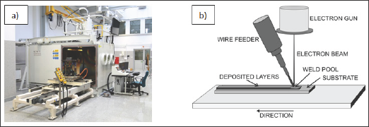
The EBAMW process was conducted based on EB machine CVE XW150 model: 30/756 (Figure 1). The device is equipped with a wire feeder and a working chamber with a volume of 4.9m3. The device is equipped with a system to monitor and record of the process parameters. The following parameters were applied during experimental tests: feeding angle 30°, working pressure 5•10-5mbar, beam current in the range of 1-30mA, accelerating voltage from 60 to 150kV, wire feed rate from 600 to 3600 mm/ min, travelling speed from 200 to 7000mm/min. To an additive manufacturing specimens welding wire 1.2mm in diameter (LNM307 Lincoln Electric: C 0.07%, Mn 7.1%, Si 0.8%, Cr 18.6%, Ni 8.0% wt.) was applied.

Figure 1: Electron beam additive manufacturing with wire set up a) EB machine b) scheme of the process.

Lupinepublishers-openaccess-journals-Civil-engineering-Architechture

Results and Discussion

The scope of the work was to investigate the influence of technological parameters such as: wire feed rate, beam current, travelling speed, acceleration voltage on stability of the deposition process and geometric dimensions of the padding welds, single layer as well as whole structure. The research revealed that, at low beam currents, the deposition process is unstable. The padding weld reinforcement is non-uniform. Irregularity of the width, height and straightness of the padding welds can be observed. At too high acceleration voltage and beam current, burn-through of plate and excess penetration weld can be revealed. When the wire feed rate is too high, the amount of energy supplied is insufficient to stabilize the fusion process of the wire. The wire is deeper feeding into the welding pool and limits the possibility of creating of a channel. The increased volume of filler material flooded the channel and caused that the welding pool becomes wider.

The gained knowledge as well as results of preliminary experimental tests including study of influence of technological parameters on with and high of single padding welds allowed to produce the fully dense metallic parts based on electron beam additive manufacturing process with wire. The results are presented in Figure 2. The EBAM 307 steel plate was fabricated in a vacuum chamber. The deposited path was scanned in one direction. It means that the return movements in opposite direction were dead. The spacing between two adjacent tracks (overlap) was 1.3mm. The scanning directions were alternated layer to layer and the time interval is 2 min. Eighteen layers were deposited and average height of each layer was approximately 1.0mm. The following technological parameters were applicable: accelerating voltage U=60kV, beam current 15mA, travelling speed 1000mm/ min, wire feed rate 1000 mm/min, feeding angle 30°. Number of padding welds in one layer was 42 [5].

Read More About Lupine Publishers Journal of Civil Engineering and Architecture Please Click on Below Link https://lupinepublishers-civilengineering.blogspot.com


Tuesday, 10 August 2021

Lupine Publishers| Beneficial Use of Nano-Silica in Concrete: A Review

 Lupine Publishers| Trends in Civil Engineering and its Architecture (TCEIA)


Abstract

   Nano-silica and its use in cement-based materials, especially concrete, has been the focus of many scientific studies. This is because cement production is an energy-intensive process and because concrete is the most used construction material worldwide. Accordingly, it is very important to understand the complexity of concrete, improve its performance and durability. This paper reviews the existing literature on the effects of nano-silica on concrete mechanical properties, microstructure and cement hydration.

Abbrevations: NS: Nano-Silica; SEM: Scanning Electron Microscopy; XRD: X-ray diffraction; FTIR: Fourier transformation infrared spectroscopy; TGA: Thermogravimetric analysis; ASR: Alkali-Silica Reaction

Introduction

The use ofnanomaterials in construction is progressively gaining popularity for the last few decades since they show significant enhancements in materials' performance. Recent studies helped to improve our understanding of nano-silica's role in the cementitious matrix. This includes cement hydration, mechanical properties and microstructure of concrete. Some of these effects are still not fully understood however. This also involves the characterization of the nano-structure of cementitious matrix in order to evaluate its effects on concrete performance using advanced characterization techniques. Furthermore, the manipulation of the nano-structure of the cementitious matrix can create superior qualities like enhanced mechanical properties, reduced porosity and even self-healing capabilities [1-3]. Further information on the importance and the problems related to the use of nanotechnology in concrete is available in the literature. In recent years, researchers investigated the effects of using nano-silica (NS) in cement pastes [4], mortars [5] and concrete [6]. They found that using small dosages of NS improves the early age and the 28-day strength gain which is attributed to the accelerating effect, pozzolanic reaction, reduced porosity and enhanced interfacial transition zone [7-9].

Effect on Mechanical Properties and Porosity

The mechanical properties of cement mortars containing nano particles specifically nano-SiO2 and nano-FeO3 were studied by Hui Li et al. [10] They observed that mortars with nano-SiO2 and nano-FeO3 achieved higher compressive and flexural strength as compared to the reference samples. Scanning Electron Microscopy (SEM) imaging revealed that nano particles did not only act as fillers but also improved the microstructure of the cement paste and promoted cement hydration. Supit, Shaikh [11] examined the durability of high-volume fly ash concrete incorporating NS. They concluded that using NS improved the compressive strength even at small replacement ratios. Moreover, the study showed that replacing 2% and 4% of cement by NS resulted in similar performance. The porosity and chloride permeability were significantly reduced after using 2% NS as compared to when only 15-20% fly ash was used. NS was also found to improve, even at small replacements, the interfacial transition zone along with the shrinkage performance.

Said et al. [12,13] found that using small dosages of NS in concrete enhanced the mechanical properties and the durability of concrete. In mixtures with 30% of cement replaced by fly ash and 3-6% NS, concrete achieved better compressive strength as compared to the mixtures without NS. Similarly, a 14% and a 32% increase in the tensile strength were observed in the mixtures when 3% and 6% NS were used, respectively. Rapid chloride ion penetration test and mercury intrusion porosimetry were used to assess the porosity. Results indicated that the addition of nanosilica significantly improves in the values of the passing charges in chloride ion penetration resistivity. Adding NS also reduced the porosity and refined the pore structure.

Effect on Cement Hydration

The characteristics of the hydration of cement mortars with NS particles were also investigated by Jo et al. [14]. Scanning electron microscopy was used to monitor the hydration and it was indicated that the addition of NS leads to improvements in the microstructure of the pastes. Mixtures with NS showed a denser, more compact micro structure as compared to Portland cement pastes that had needle-shaped hydrates which reflects the presence of calcium hydroxide. Based on these results, NS not only behaves as filler but also promotes the pozzolanic reaction.

A study by Singh et al. [15] investigated the early hydration of tricalcium silicate in the presence of NS particles. They used X-ray diffraction (XRD), Fourier transformation infrared spectroscopy (FTIR), SEM and Thermogravimetric analysis (TGA) to qualitatively and quantitatively evaluate the additional C-S-H formed. XRD results showed an increase in the intensity of C-S-H peak in the presence of NS indicating a formation of a secondary C-S-H at the early stage of hydration. A gradual decrease in the 850-950 cm-1 peak was monitored to indicate the consumption of C3S with respect to time. Their results showed that the addition of nano-silica caused an additional C-S-H formation (~50% more), accelerated the hydration and polymerization process and created a denser C-S-H.

Björnström et al. [16] studied the accelerating effects of NS on the formation of C-S-H. The diffuse reflectance FTIR spectra showed that adding NS to cement paste increased both of the consumption of C3S and the formation of C-S-H. It was found that increasing the colloidal silica from 1% to 5% by weight produced a higher acceleration effect even though smaller dosages were still considerably effective. The main conclusion was that the accelerating effects take place primarily during the initial hydration (4 - 12 hours) and that the acceleration is due to the nucleation effect of the NS particles due to their large surface area.

Effect on Durability

The use of NS to mitigate the alkali-silica reaction (ASR) in concrete was investigated by [17,18]. The study used the accelerated mortar bar testing to evaluate the performance of NS as well as its combination with fly ash and metakaolins in mitigating ASR. The study showed that NS is more effective mitigating ASR when used in combination with pozzolans such as fly ash and metakaolins. The authors attributed this to the fact that NS accelerates pozzolanic reaction, thus limiting the amount of calcium hydroxide required for ASR.

Zeidan et al. [18] investigated the effect of NS on physical salt attack. This phenomenon, which is also referred to as salt weathering, occurs in concrete in contact with soils containing high concentration of salts which gets absorbed into concrete with ground water through capillary action. Subsequently, water evaporates at the surface increasing the concentration of salts in the pores causing efflorescence and surface scaling. The study showed that adding NS to Portland cement enhanced the resistance of concrete to PSA, yet this enhancement decreased for concrete containing fly ash.

Conclusion

The use of NS is a promising approach for reducing the use of Portland cement which can help reduce CO2 footprint of construction. It was repeatedly shown that NS can enhance the properties of cement-based materials from many aspects. NS can enhance the mechanical properties of concrete, accelerate cement hydration by means of nucleation effect, and reduce porosity of cement paste through the filler action. However, further research is needed to enhance our understanding of mechanisms of concrete properties enhancements involving NS, especially in the presence of supplementary cementitious materials. Further research is needed to assess NS agglomeration and its effect on workability and means of improving its economy for widespread implementation.

Read More About Trends in Civil Engineering and its Architecture (TCEIA) Please Click on Below Link: https://lupinepublishers-civilengineering.blogspot.com

Tuesday, 22 June 2021

Lupine Publishers| Evaluation of the Performance of Asphalt Binder Modified With Nanoparticles

 Lupine Publishers| Trends in Civil Engineering and its Architecture (TCEIA)


Abstract

The physical and rheological properties of asphalt binder have been characterized using the conventional tests; (penetration, ductility, and softening point) and dynamic shear rheometer (DSR). In this study, Calcium Carbonate nanoparticles (CaCO3) and Aluminum hydro oxide (Al2O3) nanoparticles have been added to the base asphalt with a concentration of 3, 5 and 7% by the weight of asphalt. It was found that the addition of CaCO3 and Al2O3 content has a significant effect on the physical properties of the asphalt, as the penetration reduced up to 50% for modified asphalt with CaCO3 and 64% for modified asphalt with Al2O3. The softening point of modified asphalt binders was increased up to 11 and 12% for both modifiers respectively compared with the base asphalt binder. Also, the results showed that the storage stability of modified asphalt binders with CaCO3 and Al2O3 nanoparticles was less than 2.5 °C, which indicates that the asphalt binder and the modifiers having great compatibility. The evaluation of the complex shear modulus of modified asphalt binders shows that the stiffness (G*) was increased with addition increase of both modifiers, and the best performance of asphalt binder was found with the addition of 5% of both nanoparticles. As a result, the use of CaCO3 and Al2O3 nanoparticles can be considered a suitable alternative additive to modify asphalt binder.

Keywords: Calcium carbonate nanoparticles; Dynamic shear rheometer; Modified asphalt binder; Storage stability

Introduction

Asphalt is a dark brown to black cementation material in which the predominating constituents are bitumen, which occurs in nature or is obtained in petroleum processing. Asphalts are viscous liquids or solids essentially consisting of hydrocarbons and their derivatives, which soluble in carbon disulfide [1,2]. They are substantially nonvolatile at ambient temperature and soften gradually when heated. Asphalt has been used for thousands of years, and it is important as a valued engineering material continues to increase. Bitumen has been widely used in the construction of highways and road network, so in that way, asphalt should resist stresses due to traffic loads and low temperature [3]. Due to the limitation of temperature susceptibility, the low, intermediate and high temperatures and temperature performance of the asphalt need to be enhanced. Therefore, modification of base asphalt is necessary to improve the performance of material [4-6]. There are several types of asphalt modifiers, including rubbers, sulfur, polymers, fibers, and nano materials [4,7,8]. Recently, nanotechnology has rapidly been incorporated into the field of asphalt binder with different kinds of nanomaterials being used to modify asphalt and asphalt mixes. It found that nano materials can enhance the performance of asphalt binder and mixture. A study conducted by You et al. Found that nanoclay modified asphalt could reduce the strain failure rate and increase the stiffness (shear complex modulus) of base asphalt [8,9]. Also, using single-wall nano tube materials (SWNT) to modify the asphalt binder, show that the performance grade of the modified asphalt binders increased. Also, the elastic element of complex modulus of the base asphalt was less than the modified asphalts [10]. Based on the study presented by Hui Yao et al. using nano silica to modify asphalt, they found that the addition of nano silica decreases the viscosity rates of unmodified asphalt slightly. Lower and higher viscosity values of asphalt have an influential role in determining the mixing and compaction temperatures. Moreover the addition of nano silica able to reduced and delayed the aging process [11].

Experimental Design

Materials

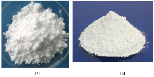
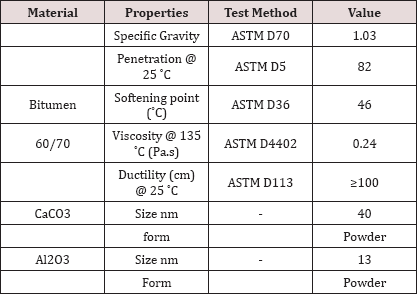
Materials were used to produce some laboratories mixed; Base bitumen binder used in this study was 60/70 penetration grade, while the nanomaterials were aluminum oxide nanoparticles (Al2O3) and Calcium Carbonate nanoparticles (CaCO3) white powder were supplied from China. The physical properties of the base bitumens binder and nanoparticles are shown in (Table 1 & Figure 1).

Figure 1: Modifiers of asphalt binder (a) Al2O3 nano particles (b) CaCO3 nano particles.

Lupinepublishers-openaccess-journals-Civil-engineering-Architechture

Table 1: Physical properties of the base asphalt and nano particles.

Lupinepublishers-openaccess-journals-Civil-engineering-Architechture

Preparation of modified asphalt binders

The base bitumen was heated to 150 °C and stirred for about 10 min, and the temperature was raised up to 170 °C. Three percentages of both modifiers (3,5 and 7% by weight) were added gradually to the base asphalt binder with constant stirring at 170 °C under the high shear mixture speed of 5000rmp for 90min until it achieves a homogenous asphalt binder blend for each percentage respectively.

Testing Procedures

Physical properties

The conventional physical tests, penetration test at 25 °C, Softening point (Ring and Ball) and ductility were conducted according to the American Society for Testing and Materials (ASTM); ASTM D5, ASTM D36, and ASTM D113 respectively.

Storage stability test

The modified asphalt cement storage stability was measured as follows. The samples were poured into an aluminum foil tube; the height of the tube is 16cm in with 3cm in diameter. The foil tubes were closed and stored vertically at a temperature of 163±5 °C in an oven for 48 hours, therefore cooled at room temperature and divided horizontally into three equal parts. The samples taken from the upper and lower sections were used to assess the storage stability of the ASA modified asphalt cement by determining the sections softening points, if the difference between the top and the bottom parts was less than 2.5 °C, then the samples were considered to have excellent high-temperature storage stability. If the softening points differed by more than 2.5 °C, the ASA modified asphalt binder was considered to be unstable [12,13].

Dynamic shear rheometer (DSR)

Dynamic Shear Rheometer (DSR) is used to determine the rheological properties of asphalt binder, including complex shear modulus (G*) and phase angle (5), at low, intermediate and high temperatures. These parameters can be used to describe both viscous and elastic behavior of asphalt. The values of G* and for asphalt binder are highly dependent on the test temperature and frequency of loading. G* is a measure of the total resistance of a material to deformation when exposed to a sinusoidal shear stress load. G* consists of both elastic and viscous components. The 5 is an indicator of the relative amounts of viscous and elastic elements. The DSR used investigates the rheological properties of CaCO3 and Al2O3 nanoparticles modified asphalt binders using a frequency sweep test. The frequency sweep applied was 0.159 to 15 Hz, and the temperatures within range 45+10 to 75 °C. One plate was used in the test, 25 mm diameter spindle with a gap of 1 mm.

Results and Discussion

Physical properties

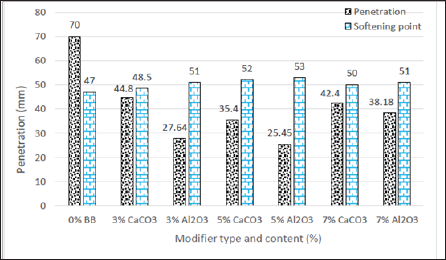
The penetration value was reduced for all modified binders at 25 °C compared with the base asphalt binder. The reduction in the penetration value for modified asphalt binders with CaCO3 was 44.8mm to 3%, 35.4 mm for 5% and 42.4 for 7% respectively. Meanwhile, it was observed that the reduction in modified binders with Al2O3 nanoparticles was. The maximum decrease in the penetration was noted with 5% for both modifiers compared with all asphalt binders. Furthermore, modified asphalt binders give a higher softening temperature compared with base asphalt binder as shown in (Figure 2). Meanwhile, the base asphalt binder has the lowest softening point temperature. The decrease in penetration and an increase in the softening point of modified asphalt binders are a result of the stiffening effect of nanoparticles. In general, the addition of nanoparticles able to enhance the properties of base asphalt up to 5% of modifier, in the meantime concentration of 7% shows different behavior as the penetration increase and softening point decreased. It might be due to agglomeration of nanoparticles during the mixing process [14].

Figure 2: Penetration and softening point of modified asphalt binders.

Lupinepublishers-openaccess-journals-Civil-engineering-Architechture

Storage stability of modified asphalt binders

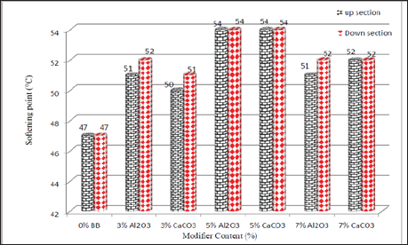
The difference in softening point values between the up and down sections of asphalt binders indicates its storage stability. The less value of the parts, the better storage stability for the modified asphalt binders [15]. (Figure 3) shows the storage stability of the base asphalt binder and modified asphalt binders. It was found that the differences in softening points in modified asphalt binders were 1 °C. Therefore, measuring the softening point of the up and bottom sections of each sample, show that the differences between the top and bottom pass the required value as it is less than 2.5 °C for all binders, this indicates that the nanoparticles modified asphalt binders were quite stable during stored at high temperatures.

Figure 3: Storage stabilities of modified asphalt binders.

Lupinepublishers-openaccess-journals-Civil-engineering-Architechture

The dynamic shear rheometer (DSR)

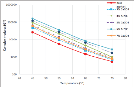
Modify of asphalt binder usually perform in two types of the binders, regarding the compatibility between asphalt and themodifier; the first one, a heterogeneous blend, the asphalt binder, and modifier are incompatible, and they are separated into two phases. The second one is a homogeneous blend, asphalt binder, and the modifier are entirely compatible [16]. The evaluation of rheological properties of modified asphalt binder shows a significant improvement in the performance of asphalt binder.binders whit Al2O3 nano particles have the highest complex shear modulus among the binders, which mean the highest resistance to deformation at elevated temperatures. Wearase, the base asphalt (Figure 4) shows that the addition of modifier increases the stiffness binder has the lowest complex shear modulus.

Figure 4: Isochronal plots of modified asphalt binders.

Lupinepublishers-openaccess-journals-Civil-engineering-Architechture

Conclusion

The evaluation of physical and rheological properties of asphalt binder shows that both modifiers have been successfully improved the physical and rheological properties of modified asphalt binders compared with base asphalt. The penetration decreased and softening point increase, which means the modified bitumen binders become harder compared with base asphalt, and the hardness of binders leads to reduce the temperature susceptibility. Also, it was found that the compatibility between asphalt and nanoparticles is significant, it might due to the uniform dispersion of nanoparticles in the asphalt blends. The result shows that 5% of both modifiers of asphalt binder can be considered as the best performance of asphalt binder.

Read More About  Lupine Publishers Trends in Civil Engineering and its Architecture (TCEIA) Please Click on Below Link: https://lupinepublishers-civilengineering.blogspot.com/


Tuesday, 20 April 2021

Lupine Publishers| A Reduced Lagrange Multiplier Method for Dirichlet Boundary Conditions in Isogeometric Analysis

 Lupine Publishers| Trends in Civil Engineering and its Architecture (TCEIA)


Abstract

Although the well-known standard Lagrange multiplier method (LMM) can even produce higher accuracy and easier implementation than other conventional schemes (e.g., the modified variational principle, the Nitsche's method), however it inherently owns many difficulties in solving the system of discretized equations, mainly caused by new unknown Lagrange multipliers. The LMM naturally increases the problem size and leads to a poorly conditioned matrix equation. The singularity is also often encountered because of inappropriate selection of interpolation space for the Lagrange multiplier. In this paper, we propose an improved method, called reduced Lagrange multiplier method, which can overcome such drawbacks raised by the LMM in treating the Dirichlet-type boundary conditions in terms of Isogeometric Analysis. By simply splitting the system equations into boundaries and interior groups, the size of system equations derived from the LMM is reduced; no additional unknowns have been added into the resulting system of equations; the Lagrange multiplier is hence disappeared; and more importantly the singular problem mentioned is avoided. The accuracy and convergence rates of the proposed method are studied through three numerical examples, exhibiting all the desirable features of the method. Optimal convergence rate and high accuracy for the present method is found.

Keywords: NURBS; Isogeometric analysis; Dirichlet boundary conditions; Lagrange multiplier method; Finite element method

Abbrevations: LMM: Lagrange Multiplier Method; IGA: Iso-Geometric Analysis; CAD: Computer-Aided DBCs: Design Boundary Conditions; DM: Direct Method; LSCM: Least-Squares Collocation Method; RLMM: Reduced Lagrange Multiplier Method

Introduction

The Isogeometric analysis (IGA) [1] employs the same computer- aided design (CAD) spline basis functions (e.g., NURBS, T-splines) to describe exact geometries and approximate physical responses. The IGA offers possibilities of integrating finite element analysis into CAD design tools and avoids mesh generation process and subsequent communication with a CAD model during refinement. The IGA has shown to be a highly accurate and robust approach for numerical simulation with exact geometry representation even with coarse mesh [2]. Moreover, the high-order smoothness of the NURBS basis functions allows for a direct construction of rotation- free plate/shell formulations [3,4] and is attractive for solving PDEs that incorporate fourth-order (or higher) derivatives of the field variable, such as the Hill-Cahnard equation [Gomez et al., 2008] [5] and gradient damage models [6].

The IGA has shown to be an effective approach in solving engineering problems as a large number of works on the theory and application of IGA have been conducted and reported in literature, including mathematical properties [7,8], integration method [9,10], spline techniques [11], fluid mechanics [12], fluid- structure interaction [13], plate/shell structures [14-17], electromechanic [18], magneto-electro elastic [19], shape optimization [20], fracture mechanics [21], and unsaturated flow problem [22]. Despite the efforts dedicated to the IGA in recent years and the significant progress has been made, some relevant technical aspects still require further studies; and among others the imposition of the Dirichlet-type essential boundary conditions (DBCs) in the IGA is an important technical issue. Given the non-interpolating nature of the NURBS basis, similar to moving least-squares [23], the properties of Kronecker delta are not satisfied, directly imposing DBCs is difficult, and special techniques are hence required.

Hughes et al. [1] addressed a direct method (DM) for DBCs enforcement to the control points. However, Wang & Xuan [24] found that the DM may induce significant errors with deteriorated convergence rates, and a special DBC treatment technique in terms of mesh less computation for contact problems [25] is presented, which is accomplished by separating the interior and boundary points on the basis of the mixed transformation method. They numerically illustrated that the improved approach produces favorable solution accuracy and optimal convergence rates compared with DM. However, the selection of boundary interpolation points should be emphasized in order to avoid a singular transformation matrix. Koo et al. [26] recently extended this method to iso geometric shape design.

Costantini et al. [27] applied the quasi-interpolation method to set inhomogeneous DBCs in the IGA on the basis of generalized B-splines to eliminate the solution of large global linear systems. Lu et al. [28] presented a technique to blend NURBS with Lagrangian interpolation in the essential boundary and allow the direct imposition of prescribed values. Other strategies based on a modified weak-form equation, such as Nitsche's method [29] and Lagrange multiplier method (LMM) have been adopted in NURBS-based IGA. Recently, De Luycker et al. [30] proposed a least- squares collocation method (LSCM) for imposing arbitrary DBCs in extended IGA. Govindjee et al. [31] later improved the LSCM by offering an efficient local least-squares algorithm to global least squares. However, LSCM is affected by the number of interpolating points. Thus, an important issue on how to choose the location and number of interpolating points precisely arises. The LMM is widely used in weak-form methods for DBCs enforcement [32].

The LMM offers solutions higher accuracy than the modified variational principle [33]. The implementation of LMM is simpler and more straightforward than the Nitsche's method [32]. However, the LMM introduces a new unknown Lagrange multiplier, which makes it difficult in selection of interpolation space for the Lagrange multiplier so that singular issues in solving the system of equations are avoided. In this paper, we present a new improved method, reduced Lagrange multiplier method (RLMM) for effective treatment of the DBCs in terms of IGA. Given that the NURBS control points can be clearly partitioned into boundary and interior groups and that the NURBS basis functions of interior control points vanish at the boundary [24], we divide the system equation of the LMM into boundary and interior groups.

Thus, the size of the equation system is now reduced and the shortcomings of the LMM can hence be overcome. Furthermore, the choice of the interpolation space for the Lagrange multiplier is studied numerically and is discussed in numerical results. The rest of this paper is organized as follows. Section 2 presents a brief on the NURBS-based IGA. Section 3 details the RLMM for essential boundary condition treatments in IGA. Numerical examples are considered in Section 4 to verify the accuracy and effectiveness of the present method. The conclusions are drawn in Section 5.

NURBS-Based Isogeometric Analysis

NURBS basis functions

In a 1D parametric space ξε[0,1], a knot vector κ(ξ) to construct the B-spline basis functions is a set of non-decreasing numbers written as Lupinepublishers-openaccess-journals-Civil-engineering-Architechture where and are the number of basic functions and the order of basic functions, respectively. Given a knot vector κ (ξ), the B-spline basis function of degree p, written as Ni,p (ξ), is defined recursively as follows [34] Lupinepublishers-openaccess-journals-Civil-engineering-Architechture


and

Lupinepublishers-openaccess-journals-Civil-engineering-Architechture

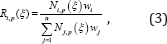
The NURBS basis function Ri,p (ξ) in the framework of partition of unity is constructed by a weighted average of the B-spline basis functions [35]:
Lupinepublishers-openaccess-journals-Civil-engineering-Architechture

where is the ith weight.

Similarly, the bivariate NURBS basis functions are expressed in the following form:

Lupinepublishers-openaccess-journals-Civil-engineering-Architechture

Where represents the 2D weight; Ni,p (ξ) and Nj,q (η) are the B-sp line basis functions defined on knot vectors κ(ξ) and κ(η) , respectively, following the recursive formula shown in Eqs. (1) and (2).

The NURBS basis functions are non-interpolatory in the interior parametric space interval. Therefore, essential boundary conditions cannot be applied simply by enforcing individual values to the control points.

By using the NURBS basis functions, a NURBS surface of order in the direction and order in the direction can be constructed as follows:

Lupinepublishers-openaccess-journals-Civil-engineering-Architechture

where Pij are the coordinates of the control points in two dimensions.

Governing equations and discretization

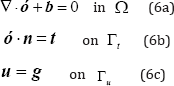
Without loss of generality, we consider a 2D isotropic elastic problem whose problem domain is with a boundary ( and ), the corresponding governing equations are expressed as follows:
Lupinepublishers-openaccess-journals-Civil-engineering-Architechture

where ∇ denotes the gradient operators; ó is stress tensor; b and t are the body and surface force vectors, respectively; n is the normal vector on Neumann boundary Γt ;g is the known displacement on Γu .

The total potential energy of the system can be constructed as follows:

Lupinepublishers-openaccess-journals-Civil-engineering-Architechture

In the NURBS-based IGA, an isoparametric concept is adopted and the NURBS basis functions are used for geometric modeling and analysis:
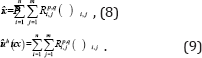
Lupinepublishers-openaccess-journals-Civil-engineering-Architechture

After the control points are rearranged with a unified subscript , the field approximation can then be written as follows:

Lupinepublishers-openaccess-journals-Civil-engineering-Architechture

where Î is the parametric coordinate; RI (Î) denotes the NURBS basis function at control point I ; NP is the total number of control points.

On the basis of the principle of minimum potential energy and by substituting the approximated displacements of Eq. (10) into Eq. (7), a system of discretized algebraic equations can be obtained as follows:

KU = f , (11)

where is the vector of the unknown variable at control points; and are the global stiffness matrix and external force vector at control points, respectively.

The element contributions to and are as follows:
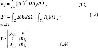
Lupinepublishers-openaccess-journals-Civil-engineering-Architechture

where D is the Hooke's elasticity matrix.

Reduced Lagrange Multiplier Method For Dirichlet Boundary Conditions

The NURBS basis functions that are often used in the IGA do not satisfy the Kronecker delta function, and the direct imposition of uI (x) = gI (x) on the control points may induce significant errors with deteriorated convergence rates [12]. The novel RLMM is presented in the following.

Reduced lagrange multiplier method

The LMM is easy to understand and implement because it has been widely used for the enforcement of DBCs. However, the LMM increases the problem size and leads to a poorly conditioned matrix equation. To overcome these shortcomings, we modify the standard LMM such that the size of the equation system is reduced. We named the modified method the RLMM. By applying the LMM, the constrained weak form is obtained as follows:

Lupinepublishers-openaccess-journals-Civil-engineering-Architechture

The matrix form of the LMM is derived as follows [Ghorashi et al., 2012]:

Lupinepublishers-openaccess-journals-Civil-engineering-Architechture

The Lagrange multiplier is approximated by the NURBS basis functions as follows:

Lupinepublishers-openaccess-journals-Civil-engineering-Architechture

The degrees of freedom (DOF) u for the control points discretized in the structure can be categorized into two groups: the constrained DOF uB that is the collection of control points ( ) for boundary description, and the unconstrained DOF uA that is the collection of control points ( ) for interior domain description. The NURBS control points can be clearly partitioned into boundary and interior groups because the corresponding NURBS basis functions associated with the interior control points vanish at the boundary. Thus, field approximation can be partitioned as follows:
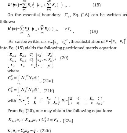
Lupinepublishers-openaccess-journals-Civil-engineering-Architechture

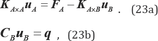
Given that the basis functions of interior control points ( NA) vanish identically at the boundary Γu ,CA =0, Eqs. (22a) and (22b) can then be respectively written as follows:
Lupinepublishers-openaccess-journals-Civil-engineering-Architechture

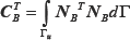
The results systems Eqs. (23a) and (23b) show that the additional unknowns, the Lagrange multiplier are disappeared, the singular problem can be avoid and the size of the equation system is actually reduced to an (n-NB) × (n-NB) matrix problem. Besides, as the NURBS basis functions are used as the interpolating functions of finite element analysis and the Lagrange multiplier (Eq.(17)), so the coefficients Lupinepublishers-openaccess-journals-Civil-engineering-Architechture is similar to a 1D mass matrix along the boundary, and the full quadrature (the number of Gauss points in each direction is p+1) is used to sure that it has an inverse.
Further discussions to the method

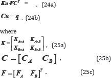
Several possibilities are available for the choice of the interpolation space for the Lagrange multiplier, such as (1) the Lagrange shape functions or (2) the same shape functions used in the interpolation of U (i.e., the NURBS basis functions in the IGA). To verify the Babuska-Brezzi stability condition and impose accurate essential boundary conditions, choosing the interpolation of the Lagrange multiplier is important. In the IGA, the matrix form of the LMM equation is expressed as follows:
Lupinepublishers-openaccess-journals-Civil-engineering-Architechture

The combination of Eqs. (24a) and (24b) perform a block-wise Gaussian elimination to obtain the pressure Schur complement as follows:

Lupinepublishers-openaccess-journals-Civil-engineering-Architechture

The question now is whether CK-1CT is invertible. K-1 is usually invertible for Laplace- and Poisson-type problems; therefore, we only need to consider whether CCT can be invertible. The Babuska-Brezzi stability condition also ensures CCT to be invertible. In the IGA, CA= 0; thus, CCT is reformed to becBcTB . If the NURBS basis functions are used as the interpolating functions of the Lagrange multiplier (Eq.(17)), then Lupinepublishers-openaccess-journals-Civil-engineering-Architechtureis similar to a 1D mass matrix, and CBCTB can be invertible. Therefore, the NURBS basis function is a stable space for the Lagrange multiplier to impose essential boundary conditions in the IGA. The NURBS basis function can obtain an acceptable solution on the numerical examples (Section 4), and the resulting system of equations will not be singular even if the number of Lagrange multipliers is large.

Numerical Examples and Discussion

In this section, three 2D examples are considered to show the accuracy and performance of the RLMM approach. The number of Gauss points in each direction is p+1 in all studies, with p being the order of the NURBS basis function. For convergence analysis, the h-refinement strategy is applied and knots are added to the middle of the knot spans. Moreover, three different measurements of error are calculated to assess the accuracy of the present method. The L2 error norm is expressed as follows:

Lupinepublishers-openaccess-journals-Civil-engineering-Architechture

where and are the exact and approximate displacements, respectively.

The H1 error norm is expressed as follows:

Lupinepublishers-openaccess-journals-Civil-engineering-Architechture

The strain energy error norm is expressed as follows:

Lupinepublishers-openaccess-journals-Civil-engineering-Architechture

where and are the exact and approximate strains, respectively; and are the exact and approximate stresses, respectively.

The exact strain energy norm is defined as follows:
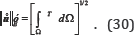
Lupinepublishers-openaccess-journals-Civil-engineering-Architechture

Laplace problem on a square domain

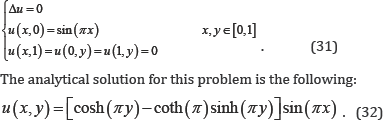
The first example considers the Laplace problem. The governing equation and the boundary conditions are expressed as follows:
Lupinepublishers-openaccess-journals-Civil-engineering-Architechture

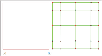
Figure 1: Initial geometry: physical mesh (a) and control mesh (b).
Lupinepublishers-openaccess-journals-Civil-engineering-Architechture

As shown in Figure 1, the initial geometry is constructed by a NURBS surface of order p = 3 for both directions with unit weights. The initial parameter space is given by knot vectors κξ = {0,0,0,0,0.5,1,1,1,1} and κη = {0,0 ,0,0,0.5 ,1,1,1,1} . For the convergence analysis, h-refinement is used to refine the mesh by knot insertion. The refined meshes have 16, 64, 256, and 1024 elements (Figure 1).

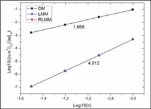
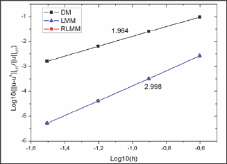
The convergence results of the RLMM, LMM and the DM are shown in Figs. 2 and 3, respectively. The optimal convergence rates are obtained for the present method and LMM while the results based on the RLMM are identical to those from the LMM. A quadratic convergence rate in the L2 error norm and a cubic convergence rate in the H1 error norm are obtained that are comparable with the quadratic convergence rate in both cases for the direct imposition of boundary conditions. We can also predict that the RLMM can compute faster than traditional LMM because only an (n-NB)x(n- NB) matrix problem (Eq.23) needs to be solved in the former rather than an ill-conditioned (n+NB)x(n+NB) matrix problem [Eq. (16)] in the latter.

Table 1: Comparison of the DOFs and condition number used for the computation among different methods.

Lupinepublishers-openaccess-journals-Civil-engineering-Architechture

The comparison of different methods on the number of degrees of freedom and matrix condition number are presented in Table 1. Divided the total DOF n into boundary DOF NB and interior DOF NA, it can be seen from Eq.(23) that the RLMM owns the same number of DOF as the DM, but the boundary DOF NB is imposed directly in DM while it obtained by solving the system of equation with smaller size Eq. (23a) in the RLMM. The total number of unknowns in the LMM will be n+NB as Lagrange multiplier unknowns are equal to boundary DOF NB. On the other hand, the matrix condition number of RLMM and DM are the same as shown in Eq. (23b). As shown in Table 1, the matrix condition number of LMM is three orders of magnitude larger than the RLMM and DM which is even worse for complicated problems. In conclusion, the RLMM has the same matrix condition number as the DM but needs to solve an Eq. (23a) to get the boundary unknowns NB. Compared with Eq. (23b), Eq. (23a) is smaller and would not waste too much time. However, compared with the DM and LMM, additional unknowns and bad matrix condition number are found for the LMM.

Figure 2: Comparison of L2 error norms for Laplace problem on a square domain.
Lupinepublishers-openaccess-journals-Civil-engineering-Architechture

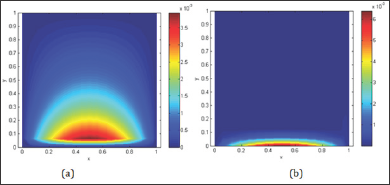
The RLMM yields the same accuracy as the LMM while avoiding bad matrix condition number as the DM and also the singularity often met in the LMM for large number of degrees of freedom is no longer encountered (Figures 2 & 3). The absolute error Lupinepublishers-openaccess-journals-Civil-engineering-Architechture distributions utilizing 256 elements are depicted in Fig. 4 to show the accuracy of the proposed approach. The following can be observed from the results: (1) the error domain derived from the RLMM is small, whereas less accuracy at the boundary can be found for the DM; (2) according to the error distributions, although the maximum value of error given by the DM is smaller than that by RLMM, the error region of DM is larger than the those of RLMM (Table 1) (Figure 4).

Figure 3: Comparison of H1 error norms for Laplace problem on a square domain.
Lupinepublishers-openaccess-journals-Civil-engineering-Architechture

Figure 4: Distributions of absolute errors obtained by (a) DM, (b) RLMM.
Lupinepublishers-openaccess-journals-Civil-engineering-Architechture

A Cantilever beam

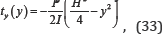
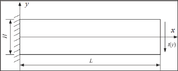
A cantilever beam with length L = 48 units and height H = 12 units subjected to a parabolic traction at the free end as shown in Fig. 5 is considered. The material properties of the beam are taken as follows: Young's modulus E = 3.0x10⁷ units, Poisson’s ratio v = 0.3. Plane stress conditions are assumed. The imposed parabolic traction is expressed by the following:
Lupinepublishers-openaccess-journals-Civil-engineering-Architechture

where I = H3 /12 denotes the moment of inertia, the shear force applied is P = 1000 units, and the left edge of the beam is clamped. The analytical displacements of this problem are given by the following [35,36]:
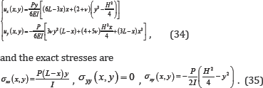
Lupinepublishers-openaccess-journals-Civil-engineering-Architechture

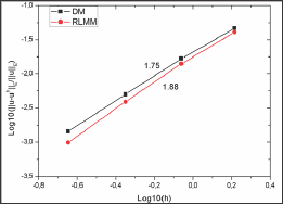
The order of the NURBS basis functions is p = 2 and the initial parametric space is defined by knot vectors . κξ=κη,={0’0’0’0.5’U’1} The weights associated with all the basic functions are set to one; thus, the NURBS basis functions are identical to the corresponding B-spline functions. The meshes used for the convergence study are 4 x 4, 8 x 8, 16 x 16, and 32 x 32 elements. The results of the L2 and strain energy error norms shown in Figs. 6 and 7 clearly confirm that the proposed method has smaller solution errors than the DM and preserve the optimal convergence rates (L2 error norm: 3.016, H1 error norm: 2.014) (Figure 5-7).

Figure 5: Description of cantilever beam problem.
Lupinepublishers-openaccess-journals-Civil-engineering-Architechture

Figure 6: Comparison of L2 error norms for cantilever beam problem.

Lupinepublishers-openaccess-journals-Civil-engineering-Architechture

Figure 7: Comparison of strain energy error norms for cantilever beam problem.
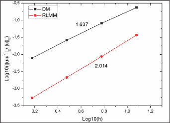
Lupinepublishers-openaccess-journals-Civil-engineering-Architechture

Infinite plate with a circular hole

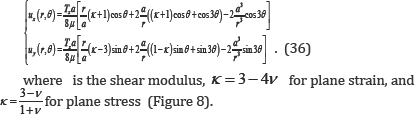
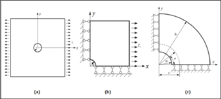
The last example deals with a plane stress infinite plate with a central circular hole under the x-direction traction Tk =1 unit (Figure 8a). Owing to geometrical symmetry, a quarter of the domain is simulated (Figure 8b). To avoid the singularity in the geometric representation, we further consider a finite annular plate in the numerical model (Figure 8c). The exact displacements using Eq. (36) are imposed on the inner and outer edges of the annular plate. The analytical displacement solutions are expressed as follows [35]:

Figure 8: Schematic description of (a) an infinite plate with a circular hole, (b) a quarter of the geometry, and (c) a finite annual plate used for numerical implementation model.
Lupinepublishers-openaccess-journals-Civil-engineering-Architechture

Lupinepublishers-openaccess-journals-Civil-engineering-Architechture

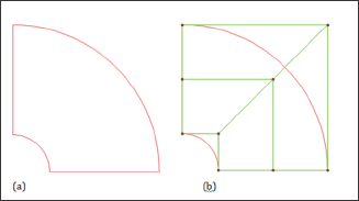
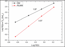
The geometry and material parameters are the radius of the circular hole a = 1 unit, the outer radius b = 4 units, Young's modulus E = 105 units, and Poisson's ratio v = 0.3. The initial geometry for this problem is shown in Figure 9. The refined meshes used in the convergence analysis are 4 x 4, 8 x 8, 16 x 16, and 32 x 32 elements. The results of L2 and the strain energy error norms are analyzed and respectively plotted in Figures 10 & 11. The proposed method has less solution errors and achieves optimal convergence rates, thus outperforming DM (Figure 9-11).

Figure 9: Initial geometry of (a) physical mesh and (b) control mesh.
Lupinepublishers-openaccess-journals-Civil-engineering-Architechture

Figure 10: Comparison of L2 error norms for infinite plate with a circular hole.
Lupinepublishers-openaccess-journals-Civil-engineering-Architechture

Figure 11: Comparison of strain energy error norms for infinite plate with a circular hole.
Lupinepublishers-openaccess-journals-Civil-engineering-Architechture

Conclusion

The Dirichlet boundary conditions (DBCs) in IGA are studied by developing an accurate treatment method, the RLMM, for overcoming the difficulties in the enforcement of DBCs. Compared with the standard LMM, the size of equation system is reduced as the resulting system of equations have made no additional unknowns, the Lagrange multipliers are thus disappeared and the singular problem in LMM is avoided. The benefit of the proposed approach can gain even greater if the number of degrees of freedom of the discretization system is relatively large. The choice of the interpolation space for the Lagrange multiplier is addressed in detail. As a result, the NURBS basis function is found to be a stable space for the Lagrange multiplier for which the DBCs in the IGA is imposed.

Nevertheless, the realization of the improved method in the treatment of DBCs in the IGA is straightforward, and can be integrated into existing IGA codes with less effort. Thus, the improved method can be ideal candidate for practical problems. Based on the numerical investigation of the convergences, the new method yields high accuracy on the solutions and optimal convergence rates, confirming the effectiveness of the enhanced treatment technique of the DBCs in the IGA. The level of accuracy and convergence rates achieved by the RLMM is better than the DM.

Acknowledgment

This work was supported by Natural Science Foundation of Hunan Province of China (2017JJ3306), Foundation of the Education Department of Hunan Province of China (17C1532), and Research Foundation of Xiangtan University (16QDZ15). The financial supports are gratefully acknowledged.

Read More Lupine Publishers Trends in Civil Engineering and its Architecture (TCEIA) Please Click on Below Link: https://lupinepublishers-civilengineering.blogspot.com/