Lupine Publishers- Environmental and Soil Science Journal
Abstract
A procedure for predicting cumulative slope displacements induced by
groundwater table changes is proposed. The proposed procedure
incorporates a back-calculation technique for the soil strength
parameter based on the records of slope displacement and ground water
table
changes. The analytical tool for the back-calculation is a
limit-equilibrium-based finite displacement method (FFDM) requiring
force and moment
equilibrium, displacement compatibility, and a hyperbolic shear
stress-displacement constitutive law. The analyzed potential sliding
mass is
a statically determinate system, providing a closed-form solution for
the displacement of the slope. Two well documented case histories of
periodic rainfall-induced slope displacements are used to validate the
proposed analytical procedures. The hyperbolic soil strength parameters
back-calculated from the first event of slope displacement can be used
as operational soil strength parameters for predicting subsequent slope
displacements caused by rainfall-induced groundwater table elevation
changes. The proposed method alleviates possible difficulties associated
with the evaluation of soil strength using undisturbed soil sampling of
colluviums in foothill areas. The proposed method requires little
computer
time in deriving useful information of slope displacement which cannot
be achieved using conventional limit equilibrium methods or advanced
numerical analyses. The proposed analytical procedure is valid only for
simulating instantaneous sliding where time-dependent viscous (or creep)
deformation is not dominant.
Introduction
A substantial part of the infrastructure damage and
remediation budget is used to fix damage caused by slope failures
[1,2]. Therefore, analyses for slope failure potential in response to
environmental changes, such as intensive rainfall, seismic activities
[3] or groundwater level changes [4] is necessary for facilitating
maintenance and disaster mitigation programs. Various analytical
methods have been developed for slope stability evaluations.
In the study of important and large-scale infrastructure such
as dams or metropolitan shield tunnels where failures are lifethreatening,
sophisticated numerical methods, such as the finite
element method (FEM) and the finite difference method (FDM),
are desirable [5]. In such cases, sufficient budgets for intensive
ground explorations, computer analysis, and skillful computational
engineers are needed. In reality, studies on slope stability are
frequently time- and budget-limited, and a numerically accurate
(or sophisticated) computer analysis often makes numerous
assumptions regarding the underground geological or geo
environmental conditions. A complete numerical analysis with
totally known material properties and underground environmental
conditions is rare. This may explain why limit equilibrium methods,
in which the displacement (or strain) is not an analytical outcome,
are still popular among geotechnical engineers in studying slope
engineering problems. Most conventional limit equilibrium slope
stability methods are based on the principle of limit equilibrium
(or force equilibrium), providing a single value of safety factor (Fs)
for the analyzed slope without considering displacement-related
information for the potential sliding soil mass. A time-efficient tool
capable of calculating slope displacements is necessary. A forceequilibrium-
based finite displacement method (FFDM) proposed
by Huang [4] is used here.
Methodology
Object of Study
The method of FFDM proposed by Huang [4] and extended by
Huang [6], Huang and Yeh [7] and Huang [8] constitutes the core
of back-calculations and predictions discussed in the following. It
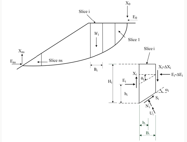
has been previously shown that for a sliced potential failure mass
confined by a slip surface with an arbitrary shape, as shown in
Figure 1, the system is a statically determinate one. A constitutive
law for the shear stress vs. shear displacement relationships based
on the hyperbolic soil model (parameters: K, n, and Rf) for the soil
constituting the slip surface is incorporated. In addition, the Mohr-
Coulomb failure criterion (parameters: cohesion, c and internal friction
angle, Ф), and local safety factor, F Si, the displacement
compatibility between adjacent slices is considered by using
displacement diagrams (displacement compatibility function f(αi)).
The vertical displacement at the top of the potential sliding mass
(D0) and shear displacement along the sliding surface (D1- Dns;
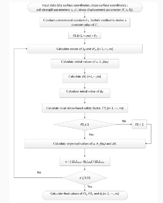
ns: total number of slices). Figure 2 shows the flow chart of the
computer program SLICE-DISP for the proposed FFDM.
Case History: Woo-Wan-Chai Slope
Figure 4: Records of long-term monitoring for case history #2: (a) Daily rainfall; (b) Groundwater table heights
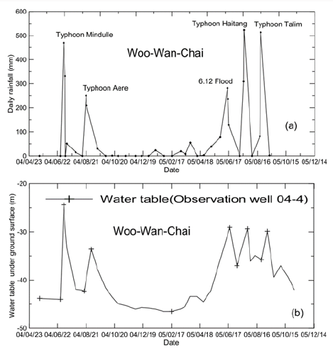

Figure 5: Conventional safety factors in response to the groundwater table fluctuations for case history #1 (Woo-Wan-Chai).
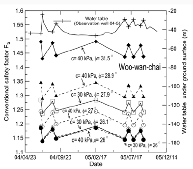

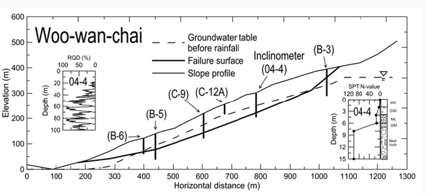
Figure 3 shows a cross section of the Woo-Wan-Chai slope
[9,10] consisting of alluviums. The slope is a part of a highway
winding through the western foothills of Taiwan. The slope is
subjected to rainfall-induced periodic displacements, requiring
repeated remedial measures. Figures 4a & 4b show records of
daily rainfall and groundwater table heights, respectively, during
the period of May 2004 to October 2005. The majority of high
daily rainfall is caused by typhoons. A close relationship between
intensive rainfalls and rises of the groundwater table can be seen.
The slip surface presented in Figure 3 is formed by connecting
points of abrupt deflection detected by the inclinometers available
in-situ. The slip surface reaches a maximum depth of about 90
m below slope surface. According to the values of Rock Quality
Designation (RQD) as shown in Figure 3, the weather rock strata
have scattered RQD values, occasionally showing a low RQD= 10%,
suggesting the investigated slip surface is associated very weak
soil-like material. Due to the difficulty associated with undisturbed
sampling in weathered rock stratum, soil shear strength can only
be estimated indirectly from the values of RQD. Values of internal
friction angles (ϕ) ranging between 260c-350c are assumed in the
following analyses. The first event of heavy rainfall (or groundwater
table rise), caused by typhoon Mindulle on July 1, 2004, is used
for calibrating in-situ soil parameters K, n, and Rf. The measured
groundwater tables before and after rainfall shown in Figure 3 are
used in the calibration of the in-situ soil parameters. Figure 5 shows
the safety factors of the slope (Fs) calculated using the Janbu’s slice
method with various input values of c and φ. It can be seen that
during the period of monitoring, values of Fs varied to some extent
according to the level of the groundwater table. However, these
values of Fs suggest that the slope is stable and thus do not reflect
the measured slope displacement.
Figure 6: Results of parametric studies on case history #1 (Woo-wan-chai) using wide ranges of K, n, c and (a) Rf=0.7; (b)
Rf=0.8; (c) Rf=0.9.
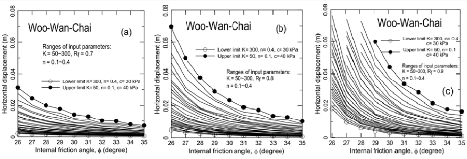
Figure 7: Records of long-term monitoring of case history #2: (a) Daily rainfall; (2) Groundwater table heights.

Figures 6(a-c) show the calculated horizontal displacement at
the location of inclinometer 04-4 (which is 280.5 m from the crest
of the slip surface) for the first rainfall event using Rf= 0.7, 0.8,
and
0.9, respectively. In Figures 6(a-c), values of K= 50, 100, 200, 300; n=
0.1, 0.2, 0.3, and 0.4; φ=260c-350c were used to account for possible
ranges of soil parameters. The reasons for using these ranges of Rf,
K, and n are given in the Discussion section. For all cases, c= 0 was
applied to the entire zone of the slope mass for the post-rainfall
condition; c= 30 kPa was applied to the above-groundwater-table
zone for the pre-rainfall condition. To obtain the calibrated values
of K, n, Rf, and φ, horizontal lines were drawn at 30 mm (measured
horizontal displacement from inclinometer 04-4 for the first event of
slope movement) in Figures 7(a-c). Values of K and n that represent
the upper bound, the intermediate value, and the lower bound of
ϕ that generate a slope displacement of 30 mm were selected as
the back-analyzed values of soil parameters. A total of seven sets
of K, n, and Rf, are used for evaluating the slope displacements
induced by the subsequent events of rainfall (or groundwater table
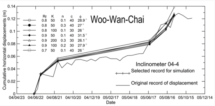
rises). Figure 8 shows a comparison of calculated and measured
cumulative slope displacements at the location of 280.5 m from
the crest of the slip surface (at inclinometer 04-4). The calculation
of cumulative slope displacements assumed that a plastic (or
irreversible) slope displacement occurs for each rainfall event. The
cumulative slope displacement measured at 280.5 m for the crest
of the slip surface is also shown. A good agreement between the
measured and calculated slope displacements (with a maximum
error of 10%) can be seen. The fact that seven sets of input K, n,
and Rf all generate similar values of cumulative slope displacement
reveals that the final results of calculation are insensitive to the
input parameters provided that the values of K, n and Rf, and φ are
calibrated using the first event of slope movement.
Case History: Ar-Li-San Slope
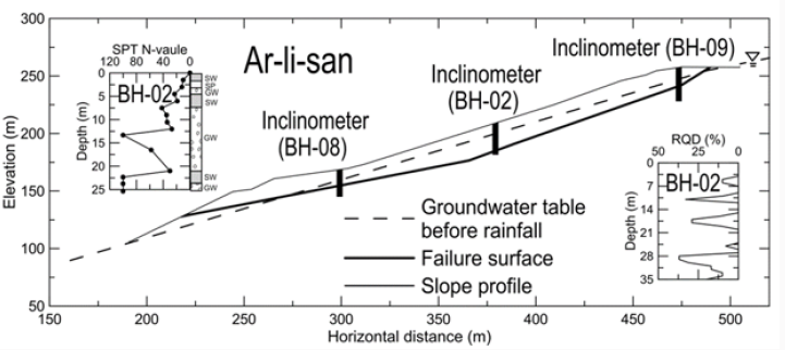
Figure 9 shows the cross section of the Ar-Li-San slope which
is on the same highway as the slope in case history no. 1 but at a
different location. A maximum depth of slip surface of about 25 m
has been detected by the inclinometers shown in Fig. 8. The borehole
data shown in Fig. 8 suggest that the slip surface locates in highly
weathered rock strata which frequently show RQD values as low
as zero. Therefore, a soil-like material is likely to prevail along the
slip surface, and φ= 250c -360c is assumed in the following analyses.
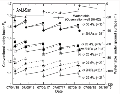
Figures 7 (a & b) show the daily rainfall and groundwater table
levels, respectively, recorded during April-August 2007. Figure 10
shows the changes of safety factors associated with the fluctuation
of the groundwater table. Figure 10 reveals a generally descending
trend of safety factors in response to the generally ascending
groundwater table during the rainy season. However, information
on the performance of the slope during the rainy season is also
lacking, as discussed for Figure 5.
Figure 11: Parametric studies for the slope displacements using various input parameters: (a) Rf=0.7; (b) Rf=0.8; (c) Rf=0.9.
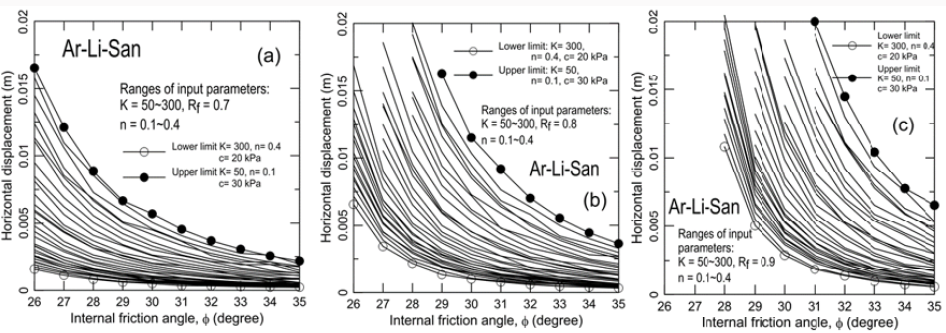

Figure 12: Comparisons of measured and calculated cumulative slope displacements for case history #2.


Figures 11(a-c) show horizontal displacements at the
location of 113 m from the crest of slip surface, calculated using
Rf= 0.7, 0.8, and 0.9, respectively. Similar to those used for case
history #1, K= 50, 100, 200, and 300; n=0.1, 0.2, 0.3, and 0.4; and
φ=260c- 350c were used. A total of nine sets of K’s, n, and Rf were
back-calculated based on an approach similar to that used in case
history no. 1 for a measured horizontal slope displacement of 3
mm from the inclinometer (BH-02) in case history no. 2. Figure
12 shows comparisons between the measured and calculated
cumulative slope displacements. The trends of all calculated
curves of cumulative slope displacement are close to that of slope
displacement during the rainy season. It can be seen that for the five
simulated events, the percentage error ranges between 10% and
20%, which is larger than that for case history no. 1 partially due to
the fact that the slope displacement in the monitoring season was
relatively small (a few mm). A 20% error for slope displacement
prediction is considered acceptable. This result confirms that the
calculated cumulative slope displacement is insensitive to the input
parameters provided that they are back-calculated from the first
event of slope movement.
Conclusion
A mechanics-based procedure for predicting continuous slope
displacements induced by periodic groundwater table changes was
proposed. A limit-equilibrium-based finite displacement method
(FFDM) previously proposed by the author was used to calibrate
soil parameters based on two long-term records of periodic slope
displacements induced by some intensive rainfall (or groundwater
table fluctuations). The proposed approach consists of a calibration
procedure that is used to find possible representative soil strength
and displacement-related parameters based on the first event of
slope movement induced by a groundwater table rise. These backcalculated
soil parameters were then used to predict subsequent
slope displacements in response to the groundwater table rise
induced by intensive rainfall. Two case histories were used to
verify the proposed approach. The effectiveness of the proposed
method in predicting groundwater-table-induced instantaneous
and cumulative slope movements was demonstrated. The proposed method
requires little computer time to provide useful slopedisplacement-
related information which cannot be achieved using
conventional limit equilibrium or advanced numerical methods.
Follow on Linkedin : https://www.linkedin.com/company/lupinepublishers
Follow on Twitter : https://twitter.com/lupine_online
No comments:
Post a Comment
Note: only a member of this blog may post a comment.