Wednesday, 31 March 2021

Lupine Publishers| Introducing DeepMind Learning Modeling

 Lupine Publishers| Advances in Robotics & Mechanical Engineering (ARME)


Abstract

Since 2010 Google & Uber researchers and engineers are engaged in DeepMind project with registered company in UK and USA DeepMind. Google used to “Deep reinforcement learning” to implement DeepMind technology. We can see the results of DeepMind learning with live examples of Google Assistance, Google Echo- Smart Speaker and Google home assistance, Google AI-God and AI Church, Amazon Alexa, Amazon echo, Apple Siri. Google is one the strong player in DeepMind learning technology but two major players also Amazon and Apple after Google. This technology brings next wave in future about to 2029 but also spoiling human ethics when AI became more then of human intelligence. This short communication discussed fundamental aspect related to DeepMind designing and engineering with the help of model.

Keywords: DeepMind; Super-AI; Ultra-AI; Bionic Brain

Introduction

DeepMind learning is the technology shift more than of AI because AI is Pre-programmed intelligence whereas DeepMind technology learn and programitself by experiences acquiring from environment and update its knowledge like human brain with more than faster of human brain. DeepMind learning is AI Deep enforcement to engineer Super-AI or Ultra-AI. Bionic Brain and Humanoid are the outstanding and breakthrough example of it. This paper shows the lucid model which assist to new entrants in the field of DeepMind and DeepMind learning. In DeepMind learning technically uses deep learning on a convolutional neural network.

Modeling

DeepMind Learning Engineering Model (DLEM)

Figure 1: DeepMind Learning Engineering Model (DLEM).

Lupinepublishers-openaccess-robotics-mechanical-engineering-journal

Below Figure 1 exhibits DLEM with further discussion of all its levels. This model segmented into two parts with equal importance as Software essential module and Hardware essential module with further segmentation into three parts of each. Both the modules and their sub-modules have further lots of depth for DeepMind engineering. Here I am not showing technical aspects in detail but would like to show direction of engineering with DLEM.

It clearly displays in above model both modules need to engineer individually but must be full interactive and suitable to each other to show human-like or more then of Human-like intelligence with proper Avatar and appearance. Software essential module has three important engineering domains are Convolution neural network Schema, Deep reinforcement learning Algorithms, GUI & Interactive Voice recognition/Interchange and interface system and Hardware essential module has Quantum Nano Memory Data structure for Neural Schemas Implementation, Robotics Sensors, Actuators and Motors for Humanoids, Robotics Violence & ethics Control System. In Software module Convolution Neural Schemas must need to engineer those has capability and ability of self-programming and learning, at Deep enforcement learning algorithms super intelligence procedure and process design to fit in neural schemas for self-learning system whereas using Human-Like GUI, Voice recognition, interaction and interchange voice command and voice response possible to/from DeepMind robots. The Second important modeling need is Hardware essential module where Quantum Nano Memory Data structure design and fabricated for Neural Schemas Implementation with ultra-high processing speed this is we can say DeepMind and Neural Schemas in it make it alive with super or ultra AI can say Bionic Brain. The next phase engineering is precision sensors, actuators and motors engineering for human like movements and appearance in humanoid. The last engineering phase is most important aspect as I mentioned Google developed AI-God and Church which volatile natural beliefs of human and one day might be DeepMind AI like this made their own AI religion and ethics which would be harmful for mankind hence need to precise Robotics Violence & ethics Control System to save human from robotics violence [1-9].

Conclusion

In above communication I had discussed about DeepMind, its concepts with current examples and using Model DLEM explained how DeepMind engineering possible to carried out. I have discussed two important engineering aspects with further expansion as well also focused on how robotics violence and ethics control system is important.

Read More Lupine Publishers Advances in Robotics & Mechanical Engineering (ARME) Please Click on Below Link https://robotics-engineering-lupine-journal.blogspot.com/


Tuesday, 30 March 2021

Lupine Publishers| Integration of Novel Emerging Technologies for the Management of Type-2 Diabetes

 Lupine Publishers| Archives of Diabetes and Obesity Journal


Introduction

The incidence of twin epidemics, obesity and type-2 diabetes are increasing rapidly worldwide in the past two decades [1-7]. By azand large, clinicians manage diabetes by meticulous management of blood glucose levels to meet the guidelines established by professional societies and regulatory agencies (8, 9). The American College of Physicians (ACP) published the most recent guideline in April of this year (8). Major guidance statements include:

a) Clinicians should personalize goals for glycemic control in patients with type-2 diabetes on the basis of a discussion of benefits and harms of pharmacotherapy, patients’ preferences, patients’ general health and life expectancy, treatment burden, and costs of care.

b) Clinicians should aim to achieve an HBA1c level between 7% and 8% in most patients with type-2 diabetes.

c) Clinicians should consider de-intensifying pharmacologic therapy in patients with type-2 diabetes who achieve HBA1c levels less than 6.5%.

d) Clinicians should treat patients with type-2 diabetes to minimize symptoms related to hyperglycemia and avoid targeting an HBA1c level in patients with a life expectancy less than 10 years due to advance age (80 years or older), residence in a nursing home, or chronic conditions (such as dementia, cancer, heart failure) because the harms outweigh the benefits in this population [8]. Recently three major professional bodies have issued guidelines on this topic. They are, American Association of Clinical Endocrinologists, American College of Endocrinology, and the American Diabetes Association [9]. In this overview (point of view), we will briefly discus some of the recent emerging technologies that may help empower and encourage patients to monitor their glucose levels and better manage their post-meal glycemic load.

According to Rebecca Voelker’s report in the recent issue of JAMA Network (May 2018), the.com Food and Drug Administration (FDA) has approved a continuous glucose monitor (CGM) that can work in tandem with mobile medical apps and automated insulin pumps to help people with diabetes manage their interstitial sugar more easily. The Dexcom G6 is the first CGM approved as both a stand-alone device and one that can be integrated into automated insulin dosing systems. According to the manufacturer, Dexcom Inc. of San Diego, California, its newly approved CGM has an easyto- use auto applicator that inserts a small sensor just beneath the skin. The sensor measures glucose levels and a transmitter inside of it sends readings wirelessly every 5 minutes to a receiver or a compatible smartphone or smartwatch. With a mobile app, users can share readings with up to 5 people. No finger sticks are needed for calibration or diabetes treatment decisions. In 2 trials, 324 adults and children aged 2 years or older with diabetes used the Dexcom G6 for 10 days. During multiple clinic visits, their readings were compared with laboratory test results that measured their blood glucose levels. An FDA statement indicated that no adverse events were reported during the studies. We would be glad to validate these sensors if the manufacturers provide them for our clinical evaluation in India.

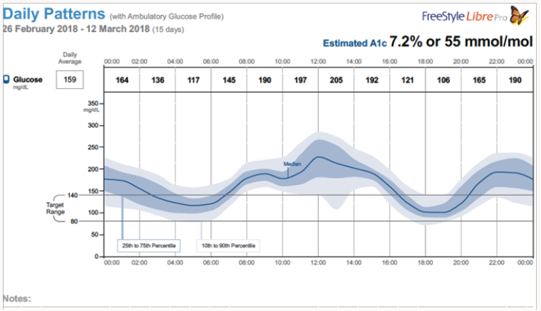
We in India are validating another CGM (Ambulatory Glucose Monitor, AGM) that is developed by Abbott Diabetes Care, Free Style Libre Pro (www.freestylelibre.com). The sensor comes with an easyto- use auto applicator. Manufacturers claim that the sensor is 48% less bulky than the Dexcom G5 transmitter and sensor. One has to use the reader that is provided by Abbott Diabetes Care. Abbott as well as iPhone do not have any apps to monitor the data from these sensors. However, android phones (with Near Frequency Communication capabilities) can read the data from these sensors. According to my collaborator Dr. Santosh, parents of type-1 diabetes patients love this system as they can keep an eye on the sugar levels of their children. To be competitive, iPhones and Abbott also should develop smart phone Apps. Abbott sensor measures glucose levels every 15 minutes for two weeks. Risk level is assessed for five time periods (there are 2 periods between bedtime and breakfast). A typical graph of median glucose is shown below. Abbott claims a strong correlation between median glucose and HBA1c (Figure 1).

Figure 1: Abbott Diabetes Care

lupinepublishers-openaccess-journal-diabetes-obesity

We are validating the usefulness or otherwise of this new glucose sensor in two independent sites in India (All India Institute of Medical Sciences, Patna, and Karnataka Institute of Endocrinology and Research, Bengaluru). The author has done some preliminary study using this sensor and a typical summary of the results are shown below. Since this study was done by an authorized endocrinologist of Karnataka Institute of Endocrinology and Research (KIER) using me as the test subject, I will refer the subject as the patient. He is (a resident of USA) over 80 years of age with well characterized type-2 diabetes for over 20 years. He is under medications (Metform in 500mg two tablets, twice daily, DPP-4 inhibitor Januvia 50mg/twice daily, Glipizide 10Mg/twice daily) and the graph shown below shows the results of a wellmanaged glucose profile. Author thanks Dr. Santosh Olety(KIER) and MS. Smitha Raja (Noesys software, Bengaluru) for these studies and analysis of the data.

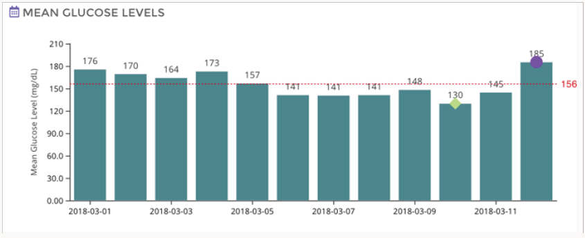
Figure 2 shows a composite data for the duration of the study (12 days). According to this data estimated HBA1c was 7.2 fairly close to the estimated clinical values. Figure 3 gives the mean glucose values for each day (variation in the mean values are not very significant). Currently, we are conducting studies to determine the correlation between the blood glucose measured by the finger prick method and the interstitial glucose measured by these emerging technologies. We also are evaluating the usefulness or otherwise of this method of glucose monitoring for the management of postmeal glucose as well as for screening of indigenous anti-diabetic drugs and their combinations.

Figure 2: Abbott Diabetes Care

lupinepublishers-openaccess-journal-diabetes-obesity

Figure 3: Abbott Diabetes Care

lupinepublishers-openaccess-journal-diabetes-obesity

As the manufacturers of glucose sensors (Dexcom and Abbott) claim, the new glucose sensors that can work in tandem with mobile medical apps and automated insulin pumps help people with diabetes manage their interstitial sugar more easily. As discussed in this overview, these sensors will serve as useful tools to manage post-meal glucose levels as well as for screening anti-diabetic drugs, dietary supplements and herbal products. Emerging technologies in device development, availability of mobile apps, improved analytics will play a very important role in the development of better affordable healthcare.

Acknowledgementment

Author thanks the following collaborators: Dr. M. A Shekar, The Director, Karnataka Institute of Endocrinology and Research (KIER), Dr. Santosh Olety, Pediatric Endocrinologist, KIER, Ms. Smitha (Raja) Bopanna, Co-Founder, Director, Noesys Software, Pvt, Ltd, Bengaluru. Dr. Sadhana Sharma, Professor, Head, Department of Biochemistry, All India Institute of Medical Sciences, Patna. Abbott Diabetes Care, Regional Representatives: Dr. Navneeth Selvan (Southern Region), Dr. Silpi Bardhan (Eastern Region).

Read More Lupine Publishers Archives of Diabetes and Obesity Please Click on Below Link https://diabetes-obesity-lupine-publishers.blogspot.com/


Monday, 29 March 2021

Lupine Publishers| Model Selection in Regression: Application to Tumours in Childhood

 Lupine Publishers| Current Trends on Biostatistics & Biometrics


Summary

We give a chronological review of the major model selection methods that have been proposed from circa 1960. These model selection procedures include Residual mean square error (MSE), coefficient of multiple determination (R2), adjusted coefficient of multiple determination (Adj R2), Estimate of Error Variance (S2), Stepwise methods, Mallow’s Cp, Akaike information criterion (AIC), Schwarz criterion (BIC). Some of these methods are applied to a problem of developing a model for predicting tumors in childhood using log-linear models. The theoretical review will discuss the problem of model selection in a general setting. The application will be applied to log-linear models in particular.

Keywords: MSE; R2; Adj R2; (S2); Stepwise methods; Cp; AIC; BIC

Introduction

Historical Development

The problem of model selection is at the core of progress in science. Over the decades, scientists have used various statistical tools to select among alternative models of data. A common challenge for the scientist is the selection of the best subset of predictor variables in terms of some specified criterion. Tobias Meyer (1750) established the two main methods, namely fitting linear estimation and Bayesian analysis by fitting models to observation. The 1900 to 1930’s saw a great development of regression and statistical ideas but were based on hand calculations. In 1951 Kullback and Leibler developed a measure of discrepancy from Information Theory, which forms the theoretical basis for criteria-based model selection. In the 1960’s computers enabled scientists to address the problem of model selection. Computer programmes were developed to compute all possible subsets for an example, Stepwise regression, Mallows Cp, AIC, TIC and BIC. During the 1970’s and 1980’s there was huge spate of proposals to deal with the model selection problem. Linhart and Zucchini (1986) provided a systematic development of frequentist criteria-based model selection methods for a variety of typical situations that arise in practice. These included the selection of univariate probability distributions, the regression setting, the analysis of variance and covariance, the analysis of contingency tables, and time series analysis. Bozdogan [1] gives an outstanding review to prove how AIC may be applied to compare models in a set of competing models and define a statistical model as a mathematical formulation that expresses the main features of the data in terms of probabilities. In the 1990’s Hastie and Tibsharini introduced generalized additive models. These models assume that the mean of the dependent variable depends on an additive predictor through a nonlinear link function. Generalized additive models permit the response probability distribution to be any member of the exponential family of distributions. They particularly suggested that, up to that date, model selection had largely been a theoretical exercise and those more practical examples were needed (see Hastie and Tibshirani, 1990).

Philosophical Perspective

The motivation for model selection is ultimately derived from the principle of parsimony [2]. Implicitly the principle of parsimony (or Occam’s Razor) has been the soul of model selection, to remove all that is unnecessary. To implement the parsimony principle, one has to quantify “parsimony” of a model relative to the available data. Parsimony lies between the evils of under over-fitting. Burnham and Anderson [3] define parsimony as “The concept that a model should be as simple as possible concerning the included variables, model structure, and number of parameters”. Parsimony is a desired characteristic of a model used for inference, and it is usually defined by a suitable trade-off between squared bias and variance of parameter estimators. According to Claeskens and Hjort [4], focused information criterion (FIC) is developed to select a set of variables which is best for a given focus. Foster and Stine [5] predict the onset of personal bankruptcy using least squares regression.

They use stepwise selection to find predictors of these from a mix of payment history, debt load, demographics, and their interactions by showing that three modifications turn stepwise regression into an effective methodology for predicting bankruptcy. Fresen provides an example to illustrate the inadequacy of AIC and BIC in choosing models for ordinal polychotomus regression. Initially, during the 60’s, 70’s and 80’s the problem of model selection was viewed as the choice of which variable to include in the data. However, nowadays model selection includes choosing the functional form of the predictor variables. For example, should one use a linear model, or a generalized additive model or even perhaps a kernel regression estimator to model the data? It should be noted that there is often no one best model, but that there may be various useful sets of variabsles (Cox and Snell, 1989). The purpose of this paper was to give a chronological review of some frequentist methods of model selection that have been proposed from circa 1960 and to apply these methods in a practical situation. This research is a response to Hastie and Tibsharani’s (1990) call for more examples.

Data and Assumptions

In this paper the procedures described here, will be applied to a data set collected at the Medical University of Southern Africa (Medunsa) in 2009. The data consist of all the tumours diagnosed in children and adolescents covering the period 2003 to 2008. The files of the Histopathology Department were reviewed and all the tumours occurring during the first two decades of a patient’s life were identified. The following variables were noted: age, sex, site. The binary response variable indicated the presence of either malignant (0) or benign (1) tumours. In our setting, the problem of model selection is not concerned with which number of predictor variables to include in the model but rather, which functional form should be used to model the probability of a malignant tumour as a function of age. For binary data it is usual to model the logit of a probability (the logit of the probability is the logarithm of the odds), rather than the probability itself. Our question was then to select a functional form for the logit on the bases of a model selection criterion such as Akaike information criterion (AIC) or Schwarz criterion (BIC).

We considered various estimators for the logit, namely using linear or quadratic predictors, or additive with 2, 3, and 4 degrees of freedom. As an alternation, the probabilities were modeled using Kernel estimator with Gaussian Kernel for various bandwidths, namely 8.0, 10.0 and 12.5. The model selection criterion that was used are AIC and BIC. Based on the above approach, recommendations will be made as to which criteria are most suitable for selecting model selection. The outline of this paper is as follows. In Section 2, we provide a brief review of the related literature. Section 3 presents technical details of some of the major model selection criteria. Some model selection methods which were applied to a data set will be discussed in Section 4. Finally, Section 5 will provide conclusions and recommendations.

Literature Review

The problem of determining the best subset of independent variables in regression has long been of interest to applied statisticians, and it continues to receive considerable attention in statistical literature [6-9]. The focus began with the linear model in the 1960`s, when the first wave of important developments occurred and computing was expensive and time consuming. There are several papers that can help us to understand the state-of-the-art in subset selection as it developed over the last few decades. Gorman and Toman [10] proposed a procedure based on a fractional factorial scheme in an effort to identify the better models with a moderate amount of computation and using Mallows as a criterion. Aitkin [11] discussed stepwise procedures for the addition or elimination of variables in multiple regression, which by that time were very commonly used. Akaike [12] adopted the Kullback-Leibler definition of information, as a measure of discrepancy, or asymmetrical distance, between a “true” model and a proposed model, indexed on parameter vector.

A popular alternative to AIC presented by Schwarz [13] that does incorporate sample size is BIC. Extending Akaike’s original work, Sugiura (1978) proposed AICc, a corrected version of AIC justified in the context of linear regression with normal errors. The development of AICc was motivated by the need to adjust for AIC’s propensity to favour high-dimensional models when the sample size is small relative to the maximum order of the models in the candidate class. The early work of Hocking [14] provides a detailed overview of the field until the mid-70’s. The literature, and Hocking’s review, focuses largely on (i) computational methods for finding best-fitting subsets, usually in the least – squares sense, (ii) mean squares errors of prediction (MSEP) and stopping rules. Thomson [15] also discussed three model selection criteria in the multiple regression set-up and established the Bayesian structure for the prediction problem of multiple regression.

Some of the reasons for using only a subset of the available predictor variables have been reviewed by Miller [16]. Miller [17] described the problem of subset selection as the abundance of advice on how to perform the mechanics of choosing a model, much of which is quite contradictory. Myung [18] described the problem of subset selection as choosing simplest models which fit the data. He emphasized that a model should be selected based on its generalizability, rather than its goodness of fit. According to Forster [9], standard methods of model selection, like classical hypothesis testing, maximum likelihood, Bayes method, Minimum description length, cross-validation and Akaike’s information criterion are able to compensate for the errors in the estimation of model parameters. Busemeyer and Yi-Min Wang [19] formalized a generalization criterion method for model comparison. Bozdogan [20] presented some recent developments on a new entropic or information complexity (ICOMP) criterion for model selection. Its rationale as a model selection criterion is that it combines a badness-of-fit term (such as minus twice the maximum log likelihood) with a measure of complexity of a model differently than AIC, or its variants, by taking into account the interdependencies of the parameter estimates as well as the dependencies of the model residuals. Browne [21] gives a review of cross-validation methods and the original application in multiple regression that was considered first. Kim and Cavanaugh [22] looked at modified versions of the AIC (the “corrected” AIC- and the “improved” AICM) and the KIC (the “corrected” KIC- and the “improved” KICM) in the nonlinear regression framework. Hafidi and Mkhadri derived a different version of the “corrected” KIC ÐKIC-) and compared it to the AIC- derived by Hurvich and Tsai. Abraham [23] looked at model selection methods in the linear mixed model for longitudinal data and concluded that AIC and BIC are more sensitive to increases in variability of the data as

opposed to the KIC

Frequentist Model Selection Criteria

Tools for Model Selection in Regression

Model selection criteria refer to a set of exploratory tools for improving regression models. Each model selection tool involves selecting a subset of possible predictor variables that still account well for the variation in the regression model’s observation variable. These tools are often helpful for problems in which one wants the simplest possible explanation for variation in the observation variable or wants to maximize the chance of obtaining good parameter values for regression model. In this section we shall describe several procedures that have been proposed for the criterion measure, which summarizes the model; These include coefficient of multiple determination (R2), Adjusted-R2 and residual mean square error (MSE), stepwise methods, Mallow’s Cp, Akaike information Criteria (AIC) and Schwarz criterion (BIC). The focus will be on AIC and BIC [24-28].

R2

Is the coefficient of multiple determination and the method to find subsets of independent variables that best predict a dependent variable by linear regression. The method always identifies the best model as the one with the largest for each number of variables considered.

This is defined as

Lupinepublishers-openaccess-Biostatistics-Biometrics-journal

Where SSE (the sum of squares of residuals) and SSY

Adjusted R - square (adj-R2)

Since the number of parameters in the regression model is not taken into account by R2, as R2 is monotonic increases, the adjusted coefficient of multiple determination (Adj - R2) has been suggested as an alternative criterion. The Adj - R2 method is similar to the method and it finds the best models with the highest Adj- R2 within the range of sizes.

To determine this, we may calculate the adjusted Rsquare. This is defined as

Lupinepublishers-openaccess-Biostatistics-Biometrics-journal

where MSY = SSY /( N −1) and MSE = SSE /(n − k) .

Mean Square Error MSE

The mean square error measures the variability of the observed points around the estimated regression line, and as such is an estimate of the error variance σ 2 . When using as model selection tools, one would calculate the possible subset of the predictor variables and then select the subset corresponding to the smallest value of MSE to be included to the final model.

It is defined as

Lupinepublishers-openaccess-Biostatistics-Biometrics-journal

where SSE is again merely the sum squared error terms and does not take account how many observations. The smaller the value of MSE, the closer the predicted values come to the real value of respond variables.

Mallows Statistics Cp

A measure that is quite widely used in model selection is the Cp criterion measure, originally proposed by C.L. Mallows (1973). It has the form:

Lupinepublishers-openaccess-Biostatistics-Biometrics-journal

where RSSp residual sum of squares from a model containing p parameters, p is the number of parameters in the model including 0 β, s2 is the residual mean square from the largest equation postulated containing all the X's, and presumed to be a reliable unbiased estimate of the error variance σ2.

R.W. Kennard (1971) has pointed out that Cp is closely related to the adjusted Rp2 and Rp2 statistic. Let us consider the relationship between adj- Rp2 or Rp2 & Cp.

Rp2 can be written as

Lupinepublishers-openaccess-Biostatistics-Biometrics-journal

where SSEp being the error of squares and SST is the total sum of squares.

The adjusted coefficient of multiple determination (Adj - Rp2),

may also be considered as:

Lupinepublishers-openaccess-Biostatistics-Biometrics-journal

Rp2 and adjRp2 is used for model containing only p of the K predictor variables. When the full model is used (all k predictor variables included) the following notation is used:

Lupinepublishers-openaccess-Biostatistics-Biometrics-journal

and the estimate of the error variance is then given as:

Lupinepublishers-openaccess-Biostatistics-Biometrics-journal

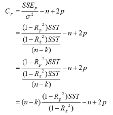
From equation (i) making SSEp the subject of the formula. It follows that

Lupinepublishers-openaccess-Biostatistics-Biometrics-journal

Substitute this into Cp

Lupinepublishers-openaccess-Biostatistics-Biometrics-journal

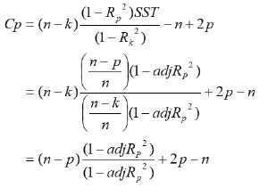
It is easily seen that Cp can be written as a function of the multiple correlation coefficient. Making (1 − Rp2) the subject of the formula from equation (3.7). It follows that in the relationship between Cp and adjR(p)2 we have

Lupinepublishers-openaccess-Biostatistics-Biometrics-journal

Then from

Lupinepublishers-openaccess-Biostatistics-Biometrics-journal

It is clear that there is a relationship between the adj-Rp2 or Rp2 and Cp statistics. In fact in both cases for each P the minimum Cp and the maximum adj-Rp2 or Rp2 occur for the same set of variables, although the P value of finally chosen may of course differ. The factor (n − k) in the first equation may cause decreases in minimum Cp values as P increases although Rp2 is only slowly increasing. Several authors have suggested using Cp as a criterion for choosing a model. We look for model with a small Cp and P preferably we look for a Cp close to P which means a small bias.

Forward Selection

In the forward selection procedure the analysis begins with no explanatory (independent) variables in the regression model. For each variable, a statistic called an F-statistic (F -to-enter) is calculated; this F-statistic reflects the amount of the variable’s contribution to explaining the behaviour of the outcome (dependent) variable. The variable with the highest value of the F - statistic (F-to-enter) is considered for entry into the model. If the F -statistic is significant then that variable is added to the model. If -statistic (F -to-enter) is greater than 10 or more, then explonatory variables are added to form a new current model. The forward selection procedures are repeated until no additional explanatory variables can be added [29-32].

Backward Elimination

The backward elimination method begins with the largest regression, using all possible explanatory variables and subsequently reduces the number of variables in the equation until is reached in the equation to use. For each variable, a statistic called an F -statistic (F-to-remove) is calculated. The variable with the lowest value of the F-statistic (F-to-remove) is considered for removal from the model. If the -statistic is not significant then that variable is removed from the model; if the F-statistic (F -to-remove) is 10 or less, then explanatory variables are removed to arrive at a new current model. The backward selection procedures are repeated until none of the remaining explanatory variables can be removed [33-39].

Stepwise Regression

Stepwise Regression is a combination of forward selection and backward elimination. In stepwise selection which can start with a full model, with the model containing no predictors, or with a model containing some forced variables, variables which have been eliminated can again be considered for inclusion, and variables already included in the model can be eliminated. It is important that the F-statistic (F-to-remove) is defined to be greater than the F-statistic (F-to-enter), otherwise the algorithm could enter and delete the same variable at consecutive steps. Variables can be forced to remain in the model and only the other variables are considered for elimination or inclusion.

Akaike Information Criterion (AIC)

Akaike (1973) adopted the Kullback-Leibler definition of information I(f;g), as a measure of discrepancy, or asymmetrical distance, between a “true” model f and a proposed model g, indexed on parameter vector Θ . Based on large-sample theory, Akaike derived an estimator for I(f;g) of the general form:

Lupinepublishers-openaccess-Biostatistics-Biometrics-journal

where the first term tends to decrease as more parameters are added to the approximating family g(y/Θ) The second term may be viewed as a penalty for over-parameterization.

Akaike Information Criterion (AIC)

Bayesian Information Criterion (BIC) Bayesian information criterion (BIC) was introduced by Schwartz in 1978. BIC is asymptotically consistent as a selection criterion. That means, given a family of models including the true model, the probability that BIC will select the correct one approaches one as the sample size becomes large. AIC does not have the above property. Instead, it tends to choose more complex models as for small or moderate samples; BIC often chooses models that are too simple, because of its heavy penalty on complexity.

A model, which maximizes BIC is considered to be the most appropriate model.

Lupinepublishers-openaccess-Biostatistics-Biometrics-journal

Where L is the maximum log likelihood, k is the number of free parameters and n is the number of independent (scalar) observation that contributes to likelihood. Model selection here is carried out by trading off lack of fit against complexity. A complex model with many parameters, having large value in the complexity term, will not be selected unless its fit is good enough to justify the extra complexity. The number of parameters is the only dimension of complexity that this method considers than AIC, BIC always provides a model with a number of parameters no greater than that chosen by AIC.

Methods

In this paper the data were partitioned into 13 sites and models fitted independently to each site. This was partially motivated during a personal discussion with Sir David Cox of the University of Oxford, who suggested that the tumours at different sites may in fact be different diseases, and therefore, may require different models for the logit of the probabilities of malignant tumours. The response variable indicated the presence of either malignant or benign tumours and is therefore a binary response. The task was now to model the probability of a malignant tumour in terms of patient age. The modern regression theory indicates that the logit of these probabilities, rather than the probabilities themselves, should be modelled either by a General Linear Model (GLM), Generalized Additive Model (GAM) or a Kernel Smooth.

At each of the 13 sites, the logit of the probabilities was modelled by increasingly flexible predictors namely: A GLM using linear or quadratic predictors, a GAM with 2, 3, and 4 degrees of freedom and a Gaussian Kernel smooth using various bandwidths, namely 8.0, 10.0 and 12.5. These are summarised in Table 1. In order to select which of the above model predictor combinations was the best at each site, we applied the model selection criteria AIC, BIC and AICc. All models were fitted using S-plus 4.0 for the purpose of assessing the models in this study. The routines for computing AIC, BIC and AICc in S-plus are given in Appendix 1 to 13. The model selection criteria, AIC, BIC and AICc were computed for each of the models described in Table 1 at each site. The model with the smallest value of AIC, BIC and AICc was then selected as the best model at a particular site. Because the Kernel smooth is a non-parametric regression without distributional assumption, it does not have a likelihood function associated with it. Because of this, the model selection criteria AIC, BIC and AICc, all of which require a likelihood, cannot be computed. We have used Kernel estimators as a non- parametric check on the best model selected from the GLM’s and GAM’s.

Table 1: Table showing the predictors that were considered for each of the various models.

Lupinepublishers-openaccess-Biostatistics-Biometrics-journal

Results

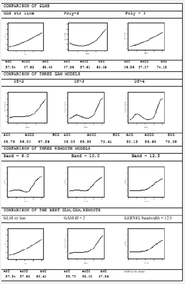
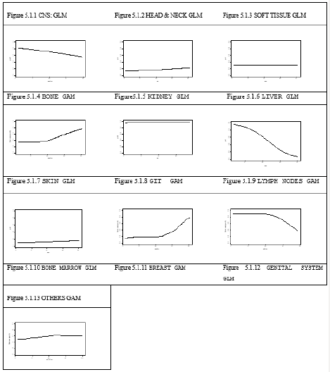
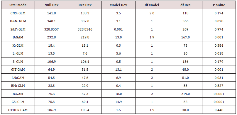
This section provides a detailed analysis of site 8 (Figure1) and a summary of the best models that were fitted at each of the best sites. This was done through presentation and discussion of the fitted models using graphs (Figure 2) followed by the analysis of deviance for each of thse fitted models as shown in Table 2. Detailed statistics for the other sites are given in Appendix 1.

Figure 1: Comparison of the estimated probability model fitted at GIT.

Lupinepublishers-openaccess-Biostatistics-Biometrics-journal

Figure 2: Graphs of estimated probabilities of malignant tumours for the best model at each of the13 sites using either a GLM or a GAM.

Lupinepublishers-openaccess-Biostatistics-Biometrics-journal

Detailed Analysis of Site 8 (Genital Internal Track)

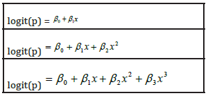
Consider the first row of model in Figure 2 which represents the GLM using respectively a linear, quadratic and cubic predictor i.e

Lupinepublishers-openaccess-Biostatistics-Biometrics-journal

For these three models, using AIC, BIC and AICc as the model selection criteria, the GAM with 2 degrees of freedom was the selected model. In Figure 2 the first row provides a comparison of the GLM’s using a linear, quadratic and cubic predictor. Both the linear and cubic predictor appears to give similar reasonable results. The quadratic predictor, however, seems to have too much forced curvature in the left-hand corner which appears to be contrary to medical experience. The second row provides a comparison of GAM’s using 2, 3, and 4 degrees of freedom respectively. The models with 3 and 4 degrees of freedom appear to have too much force curvature. The Gaussian Kernel smooth for bandwidth of 8.0 and 10.0 shows jubias curve that cannot reflect the probabilities observed in real life. The third row provides a comparison of the three final curves selected as the best fitted model from the GLM, the GAM and the Kernel Smooth. Based on the AIC, BIC and AICc criteria we have selected the GAM with 2 degrees of freedom values that are listed below the graph. It can be seen from the graph that although this has the minimum value of AIC, it is highly constrained by linearity of the predictor. The Kernel Smooth, however, is much more flexible and therefore more able to follow the data. The Kernel Smooth also seems to indicate that the logit may not be linear.

Discussion

Central Nervous System (Figure 2). The graph conveys that the probability of a malignant tumour starts from 80% at birth and decreases to 50% at age 20. The majority of tumours are malignant primitive neuroectodermal tumours and there are few benign tumours. As the children become older, the increase in astroeytic tumours remain few.ss The model deviance is 3.5 on 2.0 degree of freedom with the p=0.174 Therefore we concluded that the model is not significant for the deviance. Head and Neck (Figure 2). It starts from 10% for infants and increases to 20% for teens. The majority of these tumours are benign haemangiomas and lymphangionias.

Very few malignant tumours occur in this area. The model deviance of 3.1 on 1 degree of freedom with a p= 0.078 which is not significant (Table 2). Therefore, the model is not significant for reducing the deviance in head and neck. Soft tissue (Figure 2) There is no change of the probability of a malignant tumour from infants to late teens. The majority of these tumours are benign, which it remains constant at 30%. Soft tissue sarcoma is rare. The commonest tumours are lymphomas and haemangiomas. The model is not significantly different from the null model of constant probability: The model deviance is 0.001 on 1 degree of freedom with a p= 0.974. Therefore, we concluded that the model is not significant for the deviance. Bone (Figure 2) The probability of a malignant tumour starts from 35% in early childhood and remains constant until age 10 and then rises steeply during the teens to 80% at age 20. Bone tumours are rare in infancy.

The sudden rise of the curve is caused by osteosarcoma which is common between the ages of 10 to 20 years. The model deviance is 13.0 on 1.9 degrees of freedom with a p= 0.001. Therefore, we concluded that the model explains a significant portion of the deviance. Kidney (Figure 2) There is a constant probability of malignant tumours close to 100% over all ages from early childhood to age 20. The malignant tumour are nephroblastomas. A few cases of congenital neuroblastic nephroma were seen in malignant tumour. The model is not significantly different from the null model of constant probability: model deviance of 0.3 on 1 degree of freedom with a p=0.584. Therefore, we concluded that the model is not significant for the deviance.

Liver (Figure 2) The probability curve starts from 95% for infants and steadily declines to 10% during the teen’s years. The malignant tumours are Hepatoblast, which is common before two years. This should explain the sudden decline of the curve because malignant tumours are indeed very high. The model deviance is 5.6 on 1 degree of freedom with a p= 0.018. Therefore, we concluded that the model explained a significant portion of deviance. Skin (Figure 2) There is a constant probability of malignant tumours close to 10% from early childhood to age 10 and this probability steadily rises to 20% during teen years. A few malignant tumours are present. The probability of contracting a malignant tumour such as Kaporis sarcoma is rare in children. The model deviance is 0.5 on 1 degree of freedom with a p= 0.479. Therefore, we concluded that the model does not explain a significant portion of deviance. Genital Internal Track (Figure 2) The graph conveys that the probability of a malignant tumour starts from 15% for infants and remains constant until age 13 and then rises steeply during the teens to 80% at age 20. This is consistent with the experience in medical practice that the probability of contracting a malignant tumour, at a very young age in the genital internal track is indeed very low and that there is a sudden rise of malignant tumours around the age of 13.

The sudden rise in the 2nd decade is caused by lymphomas. The model is strongly significant: The model deviance is 13.1 on 2 degrees of freedom with a p= 0.001. Therefore, we concluded that the model explains a significant portion of deviance. Lymph Nodes (Figure2) The probability curve starts from infants at 90% and remains constant until age 12 and then decreases during the teens to 40% at age 20. Tumours at a very young age are lymph nodes which are very high and there is a decrease of the probability curve at the age of 13. The commonest tumours were lymphomas. The model deviance is 6.9 on 2 degrees of freedom with a p=0.031 Therefore we concluded that the model explains a significant portion of deviance. Bone Marrow (Figure 2) There is a constant probability of malignant tumours close to 100% from early childhood to age 20 years of age. This resonates with the experience in medical practice that the probability of contracting malignant tumours is lymphomas and leukaemias that are found in malignant tumours. The model is not significantly different from the null model of constant probability. The model deviance is 0.4 on 1 degree of freedom with a p= 0.527. Therefore, we concluded that the model is not significant. Breast (Figure 2) The probability curve starts from 90% at birth and steadily declines from malignant to benign tumours and remains constant at 10% to late teens. There was only one malignant tumour at four years. This concurs with the experience in medical practice that the probability of contracting a malignant tumour increases after puberty and it is caused by fibroadenomas. The model is strongly significant: The model deviance is 18.0 on 2 degrees of freedom with a p= 0.0001. Therefore, we concluded that the model explains a signify, can’t portion of deviance.

Genital System (Figure 2) There is a constant probability of malignant tumours close to 40% from early childhood to age 10 and slightly decreases to 2% during teen years. A few malignant tumours are present. This is in line with the experience found in medical practice that the probability of contracting a malignant tumour is benign teratomas. The model is not significant: The model deviance is 14.9 on 1 degree of freedom with a p= 0.0001. Therefore, we concluded that the model is not significant for the deviance in genital system. Others (Figure 2) The graph indicates that the probability of a malignant tumour starts from 45% for infants and remains constant until age 13 and then rises steeply during the teens to 50% until age 20. Malignant tumour for this group of patients constitutes all those sites which did not have enough cases. This should include sites where childhood malignamies which are common, and they are rare. The model deviance is 1.5 on 1.9 degrees of freedom with a p-value of 0.448 (Table 2) Therefore, we concluded that the model is not significant for the deviance.

Table 2: Analysis of Deviance for best models at all sites.

Lupinepublishers-openaccess-Biostatistics-Biometrics-journal

Conclusion and Recommendation

The problem of model selection occurs almost everywhere in statistics and we are facing more complicated data sets in the study of complex diseases. Tools that are more appropriate to the problem, more flexible to use, providing a better description, should be adopted. Model selection by AIC and BIC is one of these tools. We fitted a General Linear Model, Generalized Additive Model or Kernel Smooth using AIC and BIC model selections to the binary response to model the probability of a malignant tumour in terms of patient age. The probability of contracting a malignant tumour is consistent with the experience in medical practice and is an example of how model selections should be applied in practice. The probability distribution of the response variable was specified, and in this respect, a GAM is parametric.

In this sense they are more aptly named semi-parametric models. A crucial step in applying GAMs is to select the appropriate level of the ‘‘smoother’’ for a predictor. This is best achieved by specifying the level of smoothing using the concept of effective degrees of freedom. However, it is clear that much work still has to be done, because we have found that the Kernel smooth is a non-parametric regression which is therefore does not have likelihood function associated with it. Because of this the model selection criteria AIC and BIC, both of which require a likelihood, cannot be computed. We have used Kernel estimators as a non- parametric check on the best model selected from the GLM’s and GAM’s.

Read More Current Trends on Biostatistics & Biometrics Please Click on Below Link https://lupine-publishers-biostatistics.blogspot.com/


Friday, 26 March 2021

Lupine Publishers | Handling, Processing and Utilization Practices of Milk Products in Raya, the Southern Highlands of Tigray, Ethiopia

 Lupine Publishers | Journal of Food and Nutrition


Abstract

Cross-sectional study conducted with the aim of assessing milk products handling, processing and to characterize utilization practices in dairy farmers of Ofla, Endamekoni and Embalaje highlands of Southern Tigray, Ethiopia. A total of 156 households possessing a dairy farmers, of which 47 urban, 20 periurban and 89 rural were studied using Probability proportional to size approach sample determination. Using butter as hair ointment and custom of dying white close. About 42.31% respondents sell fresh milk, 1.92% buttermilk and yoghurt, 98.08% butter to consumers of which 93.26% of them were rural respondents. Local vessels were treated with different plant materials by cleaning and smoking. Milking vessels used ‘gibar’, plastic materials and ‘karfo’, milk souring utensils ‘qurae’ made of clay pot, plastic vessels or gourd; ghee storing 66.03% respondents in plastic, 30.13% used ’qurae’ and 3.21% use stainless steel vessels. There was significant (p<0.05) difference in the use of churning vessels in the study area where 93.6% of respondents use ‘Laga’ while the others use water tight plastic vessel.

Butter handling practice, is using ‘qorie’ :- Glass, stainless steel, log, ‘gibar’, plastic and gourd. The log ‘qorie’ was best butter handling. Butter milk (‘awuso’) and spiced butter milk ‘hazo’ stored in clay pot, plastic and stainless steel of the different milk products. Plants species used to improve milk products shelf life, cleaning and smoking of utensils includes: Olea europaea, Dodoneae angustifohia and Anethum graveolens; while Cucumis prophertarum, Zehneria scabra sonder and Achyranthes aspera were naturally rough to clean grooves of the clay pot and churner. The practice could be a base line study to cope up the problems in health risks, quality, taste and shelf life of milk products. Due attention for indigenous practices could be vital to improve livelihood of farmers’.

Keywords: Milk handling and Processing, Preservative plants

Introduction

In Ethiopia, the traditional milk production system, which is dominated by indigenous breeds of low genetic potential for milk production, accounts for about 98% of the country’s total annual milk production. Processing stable marketable products including butter, low moisture cheese and fermented milk provided smallholder producers with additional cash source, facilitate investment in milk production, yield by products for home consumption and enable the conservation of milk solids for future consumption [1]. According to Lemma [2], storage stability problems of dairy products exacerbated by high ambient temperatures and distances that producers travel to bring the products to market places make it necessary for smallholders to seek products with a better shelf-life/ modify the processing methods of existing once to get products of better shelf-life. Smallholders add spices in butter as preservative and to enhance its flavour for cooking [3]. Farmers rely on traditional technology to increase the storage stability of milk products either by converting the milk to its stable products like butter or by treating with traditional preservatives [4]. Identification and characterization of these traditional herbs and determination of the active ingredients and methods of utilization could be very crucial in developing appropriate technologies for milk handling and preservation in the country [2].

The contribution of milk products to the gross value of livestock production is not exactly quantified (Getachew and Gashaw, 2001). The factors driving the continued importance of informal market are traditional preferences for fresh raw milk, which is boiled before consumption, because of its natural flavour, lower price and unwillingness to pay the costs of processing and packaging. By avoiding pasteurizing and packaging costs, raw milk markets offer both higher prices to producers and lower prices to consumers (Thorpe et al. 2000; SNV 2008). Packaging costs alone may add up to 25% of cost of processed milk depending on packaging type used. Polythene sachets are cheaper alternatives (SNV, 2008). ‘When there is no bridge, there is always other means!’ [5], that the highland dairy farmers coping mechanisms to exploit their milk products rely up on local plant endowments even though it is not quantified.

Unlike the ‘Green Revolution’ in crop production, which was primarily supply- driven, the ‘White Revolution’ in developing economies would be demand-driven [6]. In Ethiopia, particularly, the highlands of Southern Tigray, where previous research is very meagre, the dairy products, mainly milk, butter and cheese are peculiarly exploited products than any other areas since long period of time but the doubt is their extent of production in comparison to their demand, nutritional needs and economic values, that is why the objective of this paper has targeted on the main dairy products exploitation degree in relation to the livestock resource potential. Thus research objectives are :

To identify milk production practices and constraints in the study area, and

To assess milk products handling, processing and utilization practices and methods.

Materials and Methods

Description of the Study Area

The research was conducted in Embalaje, Endamekoni and Ofla Wereda of Southern Tigray, from December, 2011-February 2012. The districts are located from 90-180 km south of Mekelle city & 600-690Km north of Addis Ababa. The study area is categorized as populated highland of the country where land/household is 0.8ha. Maichew is located at 12° 47’N latitude 39° 32’E longitude & altitude of 2450 m.a.s.l, and has 600-800mm rainfall, 12-24oC temperature, and 80% relative humidity. Korem is sited on 120 29’ N latitude, 39o 32’E longitude and Adishehu is located on 120 56’N latitude and 390 29’E longitude [7].

Study Population and Sampling Procedures

Data was analyzed using SPSS & excel. Household respondent used as sampling unit in the study and sample size determination was applied according to the formula recommended by

Arsham [8] for survey studies: SE = (Confidence Interval)/ (Confidence level) = 0.10/2.58 = 0.04, n= 0.25/SE2 = 0.25 / (0.04)2= 156

Where, confidence interval=10% and confidence level=99%

Where: N- is number of sample size

SE=Standard error, that SE is at a maximum when p=q =0.5,

With the assumption of 4% standard error and 99% confidence level.

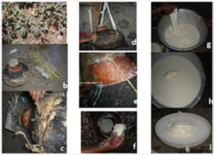
Figure 1: Act of milk processing a) Cucumis prophertarum milk vessel scrubbing b) and c), churner smoking using Anethum graveolens d) Act of churning ; e) A grass inserted in to churner (‘Laga’) to determine ripeness of butter f) g) and h) Butter separation and i) Butter bathing in water.
Lupinepublishers-openaccess-Food-Nutrition

Result

Milk Processing and Utilization Practices in Highlands of Southern Tigray

Churning: The dairy farmers practiced traditional milk processing to increase shelf life and diversify the products as soured milk, buttermilk, hazo, whey, butter and ghee that have significant nutritional, socio-cultural and economical values. ‘Laga’ hamaham (Cucurbita pepo) gourd was used in 93.6% of respondents of the study areas to churn, that could hold about 10-15 litres of accumulated milk. Procedurally Laga is washed and smoked, they heated the yoghurt to speed up butter fat globule formation, pour to the churner for churning and then let air from the churner in 15 minutes interval rest then finally, they insert a grass to check up its ripeness and pour in widen vessel to squeeze out the fat globules formed from butter milk (Figure 1). Fermented milk- yogurt “Ergo”, a traditionally fermented milk product, semi solid with a cool pleasant, aroma and flavour, used as unique medicine “tsimbahlela” during emergence and revive a person from shock and dehydration that’s why a cow is respected and considered as common resource of the surrounding in the study areas.

Buttermilk (‘awuso or huqan’) is a by-product of butter making from fermented milk. Buttermilk is either directly consumed within the family or heated to get whey/‘mencheba/aguat’ for children and calf consumption and cottage cheese known as ‘Ajibo/ayib’ for family. hazo-Fermented buttermilk with spices to extend shelf life and to provide special aroma and flavour for special occasions like socio-cultural festivals termed ‘hazo’. In holidays, 96% of dairy owners practice hazo gifts to their neighbours about a litre to each household. Even a widow who engaged in herding calves to earn weekly rebue milk, give hazo to neighbours with no milking cows. Ghee (‘Sihum’) or butter oil prepared from cows or goats milk was a special ingredient of holiday dish in majority of the dairy farmer respondents. Besides to its nutritional, ease of storage, ghee is more preferred asset for its nutrional content, ease of storage and longest shelf life, with minimum spoilage followed by butter 6 months, while shelf life of hazo is 2 weeks.

Fresh milk, yoghurt, buttermilk, whey, cottage cheese (‘Ajibo’), hazo (spiced fermented butter milk), butter and ghee (‘Sihum’) were among the common dairy products in the area with varying degree, that of fresh milk and yoghurt, were reserved for further processing, while hazo and ghee were consumed occasionally. Concerning to milk utilization, the rural household dairy farmers dominantly used the available milk for family food consumption. Dairy farmers were categorized based on marketable milk products that 98.08% of them sell butter, 77.56% of them sell fresh milk, 4.49% of them sell buttermilk and 1.92% of the respondents sell yoghurt .where as none of the respondents sell ghee, cheese, whey and hazo milk products. A farmer remarked as “honey is for a day while milk is for a year!” indicating the nutritional significance to invest for beloved family. Majority of the dairy owners were intimated with their neighbours for they do have social ties and they share animal products like the priceless life saving ‘tsimbahlela’- yoghurt during emergencies.

Milk Products Handling and Processing Vessels: Clay pot, gourds, some unreliable sourced iron and plastic containers are used for liquid milk while broad leaves like castor oil and grass weaved could serve as butter handling materials, which have sanitation problems because of grooved and irregular shapes. However, dairy farmers adapted and appreciate the rough nature of the gourds (qorie for butter storage, qurae for souring, Laga for churning and karfo for milking) and clay pots as souring and heating vessels for it absorb smoke (the disinfectant and preservative).

Milking vessels used in the study area were gibar (woven grass smeared by Euphorbia tirucelli sabs) in 9.62%, plastic jogs in 55.13% and log ‘karfo’ in 35.26% respondents. Souring vessel used by respondents was 16% clay pot, 54.5% plastic, and 29.5% gourd made of Cucurbita pepo (hamham). Ghee storage practice of the respondents was also 66.03% in plastic/ glass vessels, followed by 30.13% in clay pot termed as ‘qurae or tenqi’ and 3.21% in stainless steel vessels. gibar or agelgil was more used in Embalaje Wereda followed by Endamekoni and Ofla areas. There was significant (P<0.05) difference in churning vessel use in the study area that gourd ‘Laga’ user respondent were 93.6% while other water tight plastic vessel churner user respondents were 6.4%.

Butter handling practiced in general in ‘qorie’ type of material. Based on the respondents’ information where to store butter is stored in 2.6% glass, 6.5%)stainless steel, 7.1%log, 14.2% woven grass termed locally as ‘gibar /‘agelgil’, 17.4% plastic vessels and 52.3% gourd. Respondent remarked gourd as well insulated but difficult to in and out butter than woven grass. The log qorie was best butter handling, but not easily accessible these days because of deforestation problems that some do get from Afar region. Butter milk termed as ‘Awuso or huqan’ and spiced butter milk ‘hazo’ vessel practiced in clay pot, plastic and stainless steel. Fresh milk and butter milk boiled in stainless steel (71%) or clay pot (29%) while butter extracted in to ghee using clay pot (Table 1).

Table 1: Comparative respondents number in the study areas based on milk handling utensils.

Data in bracket indicate proportion of respondents who used the milk product vessels.

Plants used to Clean (Scrub) Vessels of Milk Products

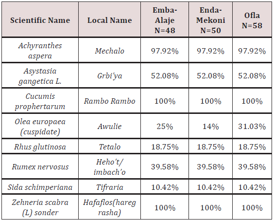
The dominant milk vessel washing herbs used in all the study areas were Cucumis prophertarum (‘ramborambo’) that prevent defragmentation of yoghurt from rarely souring problems and multi-medicinal value of their livestock, Zehneria scabra (L. fil) sonder (‘hafafelos or hareg rasha’) and Achyranthes aspera (‘mechalo’) were all rough in nature to clean the grooves of the clay pot (‘qurae’) and churner (‘Laga’) besides to their disinfectant nature. Rumex nervosus, Rhus glutinosa, and Asystasia gangetica were alternatively used. Sida schimperiana was blamed to wash clay pot which used for local brewery vessels alone, but very rare respondent argued as alternatively scrubbing vessels of milk products (Table 2).

Table 2: Plants used to clean milk product vessels in highlands of Southern Tigray.
N= Number of respondent used to practice.

Many respondent prefer Cucumis prophertarum to speed up fermentation and uniform fat texture of yoghurt. Zehneria scabra is a multifunctional herb used by many people, women in particular exploited for its medicinal value, could act as disinfectant. Olea europaea was a multifunctional tree, its leaf alternatively served to clean milk vessels that rural dairy farmers in particular 31.03% of respondents from Ofla followed by 25% respondents of Emba- Alaje, dominantly used it for scrubbing while the urban dairy respondents do have access of the dry wood to smoke. The usage of such plants along with the locally available vessels led the tradition of milk utilization practices, preferable more than technological innovation, for the immense natural aroma and flavour.

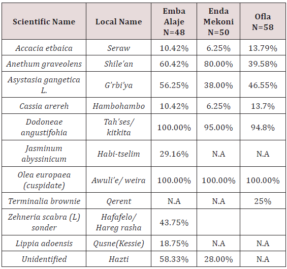
Plants used for Smoking the Milk Vessels: Three dominant plants exploited for smoking milk vessels were Olea europeana, Dodoneae angustifohia and Anethum graveolens in decreasing order in the study areas, just for fumigation, extend shelf-life, aroma and flavour due to scent scenario of the plants. Household preference and agro-ecology difference could contribute to the variety plant usage that Emba-Alaje Wereda respondents alternatively used smoke of Jasminum abyssinicum (‘habi-tselim’), ‘hazti’ and ‘qusne’ that were distinctive to the peak highlands of Tsibet and Alaje mountain chains. Accacia etbica, Asystasia gangetica and Cassia arereh were also another resource to all study sites. Optionally Terminalia brownie (‘qerenet’) was typical to Ofla Wereda (Table 3).

Table 3: Plants used to smoke milk product vessels in highlands of Southern Tigray.
NA.= Not Available

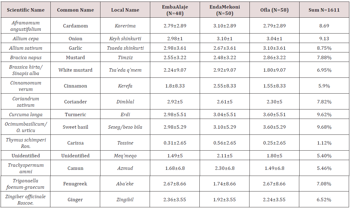
Plant Species used in Ghee (‘Sihum’) Making: The amount of spice ingredients used in ghee preparation varies from household to household according to experience and access. Curcuma longa (‘erdi’) served as colouring agent of ghee that majority of respondents deemed yellowish ghee colour is attractive. The ghee spices add value in terms of shelf-life, scene (aroma & flavour) and nutritional combinations of special ingredients (Table 4).

Table 4: Plant spices used in ghee (‘Sihum’) making in the study areas.
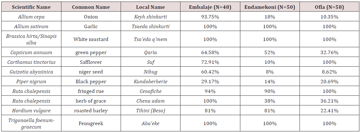
Spices used in hazo Preparation: Out of 1088 citation for hazo preparation spices (Table 5) recorded according to priority were: Allium sativum (14.34%), Brassica hirta/Sinapis alba (14.34%), Trigonaella foenum-graecum (14.34%), Ruta chalepensis (13.6%), Carthamus tinctorius (9.01%), Ruta chalepensis (8.9%), Hordium vulgar (7.26%), Capsicum annuum (6.99%), Allium cepa (5.52%), Guizotia abyssinica (3.49%) and Piper nigrum (33). Besides to ingredient value, the spices added in hazo enhance shelflife through fermentation of buttermilk.

Table 5: Plant species used in hazo making in the study areas.
Butter Packaging Practices: Based on respondents’ preference of butter packaging leaves 62.18% of the respondents used Racinus communis, 1.92% used Cassia arereh and 1.28% used Cordia africana plant leaf used as butter packaging material in the study areas. 34.62% of the respondents from urban and periurban prefer plastic package than leaves. According to some respondents the leaves were used culturally and practically for no effect over all butter property, being smooth and larger size uniformly, no butter wastage remains there, moreover, the leaf provide protection from heat. Concerning to utensil ‘qorie-log /gourd or gibar was mentioned according to their preferences based on heat protection for the butter. However, butter traders do prefer to hold on larger sized plastic pail or other stainless vessels. The effect of the packaging leaf on the quality and characteristics of butter deserves further investigation.

Discussion

The mean value of family size in the study areas 4.6±1.84 persons was comparable to CSA [7] report which was 4.5 for Endamekoni, 4.29 for Ofla and 4.36 persons for Embalaje. With the poor access of technological preservatives and processing utensils, milk products could have been perished, but many thanks to the indigenous knowledge practices of plant uses to speed up fermentation, to prevent milk spoilage and to enhance butter colour, milk products aroma and flavour supported with reports of Lemma [2]; Asaminew [3] and Hailemariam & Lemma [9].

Based on the keen observation, dauntless courage and optimism of the dairy farmers’ information, some plant such as Asystasia gangetica L. ‘giribia’ used in smoking milk utensils, just to give reddish colour of the butter, was blamed for milk bitterness that should be further investigated. Three dominant plants exploited for smoking milk vessels were Olea europaea, Dodoneae angustifohia and Anethum graveolens and the dominant milk vessel washing herbs used were Cucumis prophertarum that prevent fat defragmentation & souring problems and multi-medicinal value of their livestock, Zehneria scabra sonder and Achyranthes aspera were all rough in nature to clean the grooves of the clay pot and churner besides to their disinfectant nature. This agrees with the finding of Amare (1976); Ashenafi [4]; Lemma [2]; Asaminew [3]; Hailemariam & Lemma [9] that smoking reduced undesirable microbial contamination and enhances the rate of fermentation.

The study is similar in souring as stated by Ashenafi [4] that dairy processing, in Ethiopia, from naturally fermented milk, with no defined starter cultures used to initiate it. In many parts of Ethiopia, milk vessels are usually smoked using wood splinters of Olea europaea to impart desirable aroma to the milk. Smoking of milk containers is also reported to lower the microbial load of milk. Plant leaves of Racinus communis (‘gulei’) followed by Cassia arereh (‘hambohambo’) and Cordia africana (‘awuhi’) used as butter packaging material dominantly. The present study shows that Racinus communis and Cassia arereh are typical plant leaves to the study areas unlike Cordia africana that was reported in Hailemariam & Lemma [9] in East Shoa. Spices used in ‘hazo’ preparation were Allium cepa, Allium sativum, Brassica hirta/Sinapis alba, Capsicum annuum, Carthamus tinctorius, Guizotia abyssinica, Piper nigrum, Ruta chalepensis, Sativium vulgar, and Trigonaella foenum-graecum. Asaminew [3] reported about ‘metata ayib’ in Bahir-Dar that is relevant utilization practice of milk products.

Storage materials preference was based on their ability to retain flavour of fumigants and herbs used. Gourd ‘Laga’ or rarely water tight plastics were churning vessels of the study area unlike to clay pot churner reported by Alganesh [10] for East Welega and Asaminew [3] in Bahirdar. Alganesh reported that gourds were used commonly for storage and even for milking purpose. This indicates that the utensils used for milking, processing and storage were different from place to place and even from household to household. Efficient churning materials could contribute to lesser time and energy requirement besides to the economic return of higher butter yield for small holder dairy who do suffer from discouraging market during fasting of lent. Inefficient churner use contributed to less butter exploitation as stated by researchers (O Conner [11]; Alganesh [10]; Zelalem [5]).

Fresh milk, yoghurt, buttermilk, whey (mencheba), cottage cheese (Ajibo), hazo, butter and ghee (‘Sihum’) were among the common dairy products in the area with varying degree, that of fresh milk and yoghurt, were reserved for further processing, while hazo and ghee were consumed occasionally. The result is consistent with many of the research findings Lemma [2]; Asaminew [3] & Zelalem [5]. The limited consumption of butter may be due to the higher price associated with it and the need for cash income to buy some necessities. Butter can fetch them a good price compared to other milk products. Butter was consumed only during holidays and special occasions in rural low-income households because it fetches routine cash income Asaminew [3].

Different spices were used in ghee making. The finding was consistent with the reports of Alganesh [10] in East Wellega, Lemma [2] and Hailemariam and Lemma (2010) in East Shoa. Ghee was not marketed in the areas surveyed due to consumers’ preference to make their own ghee depending on their test and preference for different spices that the finding has close affinities with Hailemariam & Lemma [9]. Compatibly with Asaminew [3], consumers /traders consider the colour, flavour, texture and cleanness of the products during transaction, that butter quality requirements fetch a good price. During the dry seasons butter price increase, this is related to abridged milk yield of cows due to the insufficient feed supply. Higher price was also paid for yellow coloured and hard textured butter that deemed to be higher in dry matter or solid non fat for extraction consistent with reports Asaminew [3].

In the districts those smallholders who do not sell fresh milk had different reasons. These were small daily production of fresh milk, cultural barrier, lack of demand to buy fresh whole milk and preference to process the milk into other products. Similar reports were made by Alganesh [10] and Lemma [2]. Besides, it is difficult to find a market. Typical to the research observation on milk marketing problems, the Ethiopian highland smallholder produces a small surplus of milk for sale. The informal system where the smallholder sells surplus supplies to neighbours or in the local market, either as liquid milk or butter but contradict in cottage-type cheese called ayib. Sintayehu [12] selling that was unusual including buttermilk, ‘hazo’, whey, cottage cheese and ghee. In the vicinity of larger towns the milk producer has a ready outlet for his liquid milk. However, in rural areas outlets for liquid milk are limited due to the fact that most smallholders have their own milk supplies and the nearest market is beyond the limit of product durability like to many of the studies done (Getachew and Gashaw (2001); Sintayehu [12]; SNV (2008); Tesfaye et al. (2010)) besides to cultural traditions and lower talents entrepreneurship of the farmers.

Many research findings similarly stated that there were several constraints to the dairy in particular to milk marketing development, e.g. lack of infrastructure and finance, seasonality of supplies and lack of market structure and facilities [3]. Because of the lack of cooling facilities or even suitable utensils for milking and storing, milk deteriorates rapidly [11]. Milk is often sold for less than its full value due to lack of access to markets, poor road infrastructure, lack of co-operatives, inability to transport long distances due to spoilage concerns, and unscrupulous traders who add water or other fillers the study was consistent with PPLPI (2009) and cultural taboos and discouraging market [3]. Contrary to perceived public health concerns, the marketing of raw milk does not pose public health risks as most consumers boil milk that consistent was Kurwijila [13] and exploit local herbal resources to smoke and clean the milk products vessels that served as disinfectant, preservative, tasteful with natural aroma and flavour Asaminew [3] ; Desalegn [14] & Zelalem [5] before drinking it.

Conclusion and Recommendations

Livestock production plays an important role in the socioeconomic and cultural life of the people inhabiting in the mountainous chains of the area. The cows fulfil an indispensable role for the dairy farmers serving as sources drought ox, milk food, income from sale of butter, the only determinant women hair lotion, source of dunk cake fuel and served as prestige and confidence to avert risks. The respondent remarked “Wedi Lahimika -for own bull and no one could cheer you what a cow could do indeed” to mean reliable resource and do have special dignity for the cow.

Milk produced every day was collected in the collection clay pot, plastic vessels or ‘Laga’ smoked with woods called Olea europeana, Dodoneae angustifohia, Anethum graveolens Acacia etbaica, Terminalia brownie, and in some cases Cassia arereh and the dominant milk vessel washing herbs used were Cucumis prophertarum that prevent yoghurt from defragmentation during rarely souring problems and multi-medicinal value of their livestock, Zehneria scabra (L. fil) sonder and Achyranthes aspera were all rough in nature to clean the grooves of the clay pot and churner besides to their disinfectant nature. As reported by respondents, the purpose of smoking was to minimize products spoilage during storage and to give good aroma and flavor. Keeping milk or milk product for longer period without spoilage and flavor was indicated as main reasons for using plants in washing (scrubbing) dairy utensils [15].

Materials Commonly used for Milk Collection Storage and Processing included Clay Pot, Glass Container, Wooden Container, Plastic Container, Woven Materials, Plastic Container and Gourd

1. The emerging markets of buttermilk and yoghurt in farm gates should be expanded to other means of marketing systems via integrated awareness creation

2. The effect of these materials on the shelf- life of stored or preserved butter deserves further investigation. The impact of local herbs used as preservatives should be further studied [15].

3. Facilities for cleaning and overnight storage, milk churns and dairy utensils are rudimentary, requiring intervention.

Read More Lupine Publishers Food and Nutrition Journal Please Click on Below Link
https://lupine-publishers-food-and-nutrition.blogspot.com/


Thursday, 25 March 2021

Lupine Publishers | Somatic Mutations in Cancer-Free Individuals: A Liquid Biopsy Connection

 Lupine Publishers | Journal of Oncology

Abstract

Somatic mutations have been perceived as the causal event in the origin of the vast majority of cancers. Advanced massively parallel, highthroughput DNA sequencing have enabled the comprehensive characterization of somatic mutations in a large number of tumor samples for precision and personalized therapy. Understanding how these observed genetic alterations give rise to specific cancer phenotypes represents an ultimate goal of cancer genomics. However, somatic mutations are also commonly found in healthy individuals, which interfere with the effectiveness for cancer diagnostics.

Keywords: Somatic mutation; Germline; Cell-free DNA; Liquid biopsy; Next-generation sequencing

Abbreviations: NGS: Next-Generation Sequencing ; cfDNA: Cell-free DNA; MAF: Mutant Allele Frequency

Introduction

Mutations in healthy individuals are not all germline

Over the course of our lifetime, there are many millions of cell divisions in the body. By chance alone, mutations will definitely occur. Indeed, spontaneous somatic mutations constantly occur in individual cells. These background mutations arise either from replication errors or from DNA damage that is repaired incorrectly or left unrepaired, and have been detected in healthy tissues, including blood, skin, liver, colon, and small intestine [1-3]. Deepsequencing studies in normal tissues also surprisingly identified cancer-driving mutations, e.g., in blood, driver mutations can be detected in ~10%of individuals older than 65 years of age and resemble patterns seen in leukemia patients. Individuals carrying these driver mutations have an elevated future risk of blood cancers [4-6], suggesting that these are genuine precancerous clones. Further, a detailed analysis of 31,717 cancer cases and 26,136 cancer-free controls from 13 genome-wide association studies revealed that the majority, if not all, of aberrations that were observed in the cancer-associated cohort were also seen in cancer-free subjects, albeit at lower frequency [7,8].

Somatic mutations in healthy individuals are very prevalent, with an average mutation number of around 2–6 mutations/1 M bases [9,10]. The baseline somatic mutation spectrum in healthy population not only can help fill the gaps for the establishing early cancer diagnosis strategies, but also argues against the idea of using normal cells as germline control to make somatic mutation calls in sequencing tests. Moreover, the same driver mutation could exist in both tumor and normal cells yet with distinct biological effects, we should not simply define the threshold of mutation detection by removing the background mutations found in a healthy population. Taken together, we need to incorporate and carefully calibrate the background somatic mutations in healthy individuals; the fact is they are not all germline mutations.

Somatic driver mutations found in healthy population by liquid biopsy

With the dramatically decreased cost of next-generation sequencing (NGS) in recent years, it is now practical to screen a large number of individuals at ultra-deep sequencing depths to identify cancer-related mutations. Cell-free DNA (cfDNA) in the blood circulation of cancer patients (as liquid biopsy) have emerged as key biomarkers for cancer monitoring and treatment decisionmaking [11]. Both academic research groups and industry players are chasing the pan-cancer screening by a simple blood draw. However, the reliable and accurate application of cfDNA detection requires better understanding of background somatic information in healthy individuals.

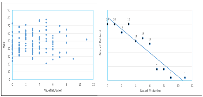
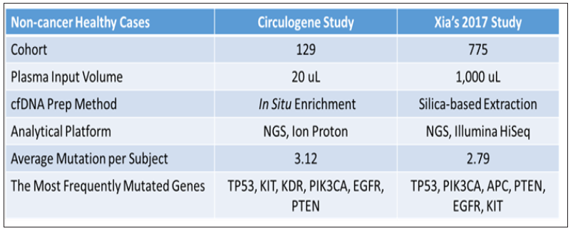
We performed ultra-deep target sequencing on 50 cancerassociated genes for plasma cfDNA from a cohort of 129 apparently healthy cancer-free subjects. To increase the confidence of the called mutations, we here defined the mutation as the variant allele frequency greater than 1% and the average depth more than 5,000 xs for demonstration. Our data revealed an age-independent mutation spectrum with average 3.12 somatic mutations per subject (Figure 1). The most frequently mutated genes are TP53 (42%), KIT (6%), KDR (5.5%), PIK3CA (5.5%), EGFR (5%) and PTEN (3.7%). These results highlighted the prevalence of some cancer-associated driver mutations in healthy individuals as background mutations. We also demonstrated the concordance between our results and a recent study for revealing the real somatic mutation in healthy population.

Figure 1: Distribution plots of somatic mutation detected in a cohort of 129 healthy subjects.

The study by Xia et al. [12] examined the background somatic mutations in white blood cells and cfDNA in healthy controls based on sequencing data from 821 non-cancer individuals with the aim of understanding the baseline profile of somatic mutations detected in cfDNA. The data comparison was summarized in Figure 2. Although there are differences in study cohort composition, sample volume, extraction methodology and analytical platform, the end results are remarkably similar, i.e., average 3 mutations per subject with an almost identical list of frequently mutated genes. Although varying mutation spectra in cancers have often been attributed to cancerspecific processes, our data suggest that at least a subset of these mutations actually reflect normal tissue-specific processes. This concept is consistent with the idea that a substantial fraction of the mutations found in cancers occur in normal stem cells [13,14].

Figure 2: Comparison of somatic mutation detection in healthy population from two studies.

Normal tissue as a germline control not justified

There is evidence for the presence of tumor-derived cfDNA in early cancers [15]. However, the real fraction of cfDNA that shed by tumor rather than the background somatic mutations is not well illustrated. For clinical application, the low level of tumor mutation as well as the heterogeneity of background mutation present in the circulation needs to be clearly addressed and differentiated to achieve accuracy. Unfortunately, this goal can’t be achieved by pushing detection limit of current advanced technology to below 0.01% mutant allele frequency (MAF). Contrarily, the higher sensitivity will guarantee higher chance to pick up background somatic mutations. Also, the clinical relevance of those lowpercentage tumor mutations is still debatable in terms of treatment decision or regimen change. Each human individual is unique. Every cancer patient is different. No two tumors are the same even resides within the same patient; to distinguish the definitive cancer-specific mutations from background signals observable in plasma is extremely daunting. Evaluation of specificity in plasma cfDNA profiles from large numbers of healthy individuals as representative controls for the cancer population seems farfetched with uncertainty, especially when standardized protocol and optimized technology are still lacking.

Unlike tissue genomic DNA, circulating cfDNA is so diluted and dynamic with a relatively short half-life, making single-point measurement not suitable for clinical application. We reason that cfDNA in circulation is truly under a continuous selection pressure to select for highly aggressive/proliferative clones, as disease progressing the low-abundant tumor clones will either evolve and dominate or vanish by the immune clean-up processes, therefore longitudinal clinical follow-up should be performed to identify the best time and target for precision therapy, meanwhile to filter out contaminating background mutations. To achieve high clinical specificity, a cfDNA-based test must be capable of distinguishing between the background signals originating from non-cancer or pre-cancerous processes and the invasive malignancy of clinical interest. It is still possible that mutational signatures in cfDNA could distinguish basic biological processes from malignant and pathological processes.

Figure 3: A representative mutational trending curve after filtering out background mutations.

Here we propose a combined approach based on the tumor evolutional principle of “survival and domination of the fittest” in circulation that is to perform multiple time-point monitoring, filter out potential background mutations (e.g., <1% MAF), reduce sample input volume and interrogate multiple databases. A representative mutational trending curve following our approaches was shown (Figure 3). Our findings underscore the importance of an assessment of the landscape of somatic mutations in cancerfree population, and associated mutation signatures. Somatic mutations and mosaicism in healthy individuals have implications not only for early detection, diagnosis and treatment of cancer using liquid biopsy but also emerging technologies in healthcare. We recommend caution while extending the mutation conclusions to cancer patients by employing matched normal tissue as germline control. To increase sample input and push liquid biopsy sensitivity toward <1% may not serve the interest of detecting low-frequency mutant allele, but only to increase the chance of background mutation contamination. Application of artificial intelligence, machine-learning on big database to create an algorithm for highrisk population screening of cancer is a good idea for preventive medicine, yet the outcome is uncertain given the uniqueness of every patient, each tumor - one size can’t fit all.

Read More Lupine Publishers Oncology Medicine Journal Please Click on Below Link
https://lupine-publishers-cancer-journal.blogspot.com/