Showing posts with label International Journal of Otolaryngology. Show all posts

Tuesday, 22 November 2022

Lupine Publishers| Nasolabial Cyst: Report of 2 Cases and Literature Review

 Lupine Publishers| Journal of Otolaryngology


Abstract

Introduction: Nasolabial cysts are a rare, ectodermal development cyst, presenting as a fullness of canine fossa, nasal ala or vestibule of the nose. They are usually asymptomatic but may become infected. Treatment is complete surgical excision by sublabial approach, or transanal endoscopic marsupialization.

Case Report: Description of two cases, one female presenting as nasal deformity due to progressive growth of unilateral nasolabial cyst, and a healthy young male presenting severe facial cellulitis, with a CT showing bilateral nasolabial cysts.

Discussion: Nasolabial cyst is a rare condition, but diagnosis and treatment are simple. Nasolabial cyst should be incorporated by ENT in the differential diagnosis of nose deformities and facial swelling.

Introduction

Nasolabial cysts are also described as nasoalveolar cyst or Klestadt cyst and were first described by Zuckerkandl [1,2]. They are rare, affecting 1,6 per 100.000 persons per year, more frequently in females (4:1 ratio), especially among African Americans, in the fourth and fifth decades of life. 90% are unilateral, and often underdiagnosed [3,4]. Nasolabial cysts are non-odontogenic cysts that develop lateral to the midline of the maxillary lip and alar base. They usually present as a swelling in the nasolabial fold, causing alar nose elevation and upper lip projection. They may grow slowly and painlessly over several years. Because of its close anatomical relation to the nasal cavity and teeth, they may become infected easily, rapidly growing and being painful [1,5]. Diagnosis is made by clinical examination, imaging tests, and is confirmed by histopathologic study. The cyst can be palpated bimanually with one finger in the floor of the nasal vestibule and another in the labial sulcus. Computed tomography (CT) and magnetic resonance (MR) can be useful. Differential diagnosis includes cysts of the nasopalatine duct, periapical inflammatory lesions (granuloma cyst, abscess), and epidermoid cysts [1,6]. Complete surgical excision of the nasolabial cyst is the best treatment, and sublabial approach is most used. Other authors propose transanal marsupialization as an easier and shorter procedure, with lesser complications, but recurrence may be a problem [3,5].

Case Report 1

Figure 1(a).

lupinepublishers-openaccess-journal-otolaryngology

Y=372.256 + 6.8856. X1+residuals

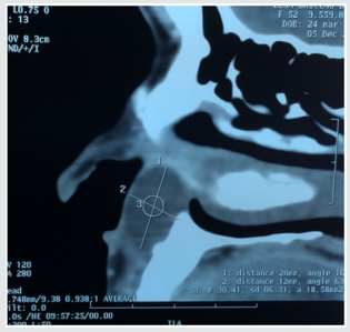
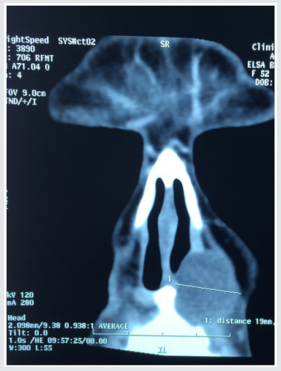
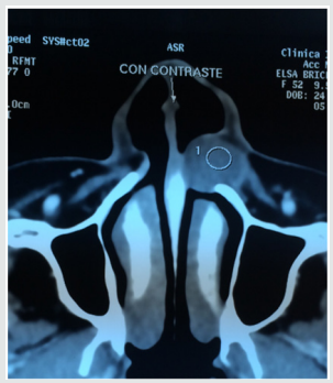
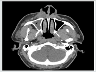
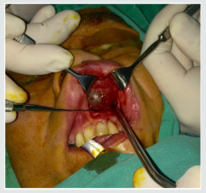
52-year-old female patient with a 3-year history of left floor of nose intermittent painful swelling, and progressive deformity of this area. Computed tomography (CT) study showed a 3,2 cm rounded lesion in left pyriform aperture compatible with nasoalveolar cyst (Figure 1). A sublabial approach was performed, and complete excision of the cyst was obtained (Figure 2). Histological study confirmed suspected diagnosis. Patient evolved in excellent conditions, with no complications or recurrence in a 2 year follow up period.

Figure 1(b).

lupinepublishers-openaccess-journal-otolaryngology

Figure 1(c).

lupinepublishers-openaccess-journal-otolaryngology

Figure 2. Intraoperative view of sublabial access to left nasolabial cyst in Case 1.


Case Report 2

Figure 3. Computed tomography of bilateral nasoalveolar cysts. Case 2.

lupinepublishers-openaccess-journal-otolaryngology

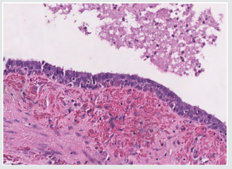
Figure 4. Pathology H-E study of Case 2 showing cyst wall with pseudostratified columnar cells.

lupinepublishers-openaccess-journal-otolaryngology

37-year-old male patient, with no prior medical record, developed a facial cellulitis with no initial response to oral antibiotics, requiring hospitalization and intravenous antibiotic treatment. Maxillary and orbital CT study showed bilateral nasoalveolar cysts, with signs of active infection in the right cyst (Figure 3). Antibiotic treatment was completed, and cyst resection was programmed a month later. An extensa sublabial approach was performed, and bilateral cysts were removed. Histological findings confirmed diagnosis (Figure 4). Patient did not have any other episode of facial cellulitis or cyst recurrence in a 14 month follow up

Discussion

Origin of nasolabial cysts is controversial. Most accepted theories are that cysts derive from remnants of the nasolacrimal duct or inclusion cysts of mesenchymal cells during the fusion of medial and lateral nasal prominences to the maxillary prominence during facial skeletal formation [2]. Histology usually present pseudostratified columnar epithelium. Su et al noticed with electronic microscopy that that cysts had a highly placated mucosa, of non-ciliated stratified columnar epithelium, differing from the ciliated columnar epithelium of the paranasal and nasal sinuses [7]. The treatment of nasolabial cysts consists on complete removal of the lesion, with the objective of prevention of infectious complications, histologic diagnosis, and aesthetic improvement. Fine needle aspiration can help in diagnosis, and relieve of symptoms, but recurrence is high [1]. Surgery is usually done by sublabial approach, creating a mucosal flap of gingiva to allow access to the pyriform aperture and to the cyst, which can be resected carefully to avoid rupture, especially to the floor of the nose mucosa, and complete excision is mandatory to avoid recurrence. After the intervention, the gingival mucosal flap is fixed in its original position with absorbable sutures. Potential complications are uncommon, including facial swelling, insensitive gingiva, teeth numbness, and surgical site infection.

Patients must use a toothbrush on the surgical site. Diet should be soft for the first week, then normal. Dental prostheses can be used immediately after surgery [1]. Lee et al published in 2009 a comparative study between surgical techniques, and strongly suggested endoscopic trans nasal marsupialization as a simpler, shorter and safer procedure, and in most cases, it could be done under local anesthesia [3]. In our two cases we used sublabial approach with general anesthesia because is the usual technique used in our practice, but we are interested to use endoscopic marsupialization in next cases. We did not have any complications or recurrences in follow up of both cases.

Conclusion

Nasolabial cysts are rare but must be considered in the differential diagnosis of floor of the nose deformities and facial swelling. Sublabial approach is the most common procedure, but probably be replaced by endoscopic marsupialization in the future.

Read More About Lupine Publishers Journal of Otolaryngology Please Click on Below Link: https://lupine-publishers-otolaryngology.blogspot.com/

Saturday, 6 February 2021

Lupine Publishers | Categorical Loudness Scaling in the Fitting of Cochlear Implanted Children

 Lupine Publishers | Journal of Otolaryngology


Abstract

The correct - optimal - fitting of speech processor determines the best result of rehabilitation. The optimal setting of most comfortable level (MCL) is achieved by accurate patient’s assessment of electrical stimuli loudness. Unfortunately, small children can’t give a reliable report about their feelings. How to determine the MCLs in every channel of children implant? Objective methods don’t give the final (optimal) comfort levels of the child’s working program. Therefore, we need subjective assessments. We tried to use a method of categorical loudness scaling (CLS). This article is a guide how to teach CI children to evaluate loudness. Good results of the CLS were observed.

Keywords: Cochlear Implant; Fitting, Categorical Loudness Scaling; C – Levels; Most Comfortable Levels (MCLS); Threshold Discomfort Levels

Introduction

The correct (optimal) fitting of the processor determines the best result of rehabilitation [1]. The optimal settings of C-levels are achieved by accurate subjective patient’s assessments of the electrical stimuli loudness. Unfortunately, young children cannot give a verbal report about their feelings. How to determine the maximum comfortable levels (MCLs) in every channel of an implant in children, i.e. to find threshold discomfort levels? For example, an objective method – reflexometry (registration of stapedial reflex) – is used for fitting of children. But the program in which MCLs are equal to the reflex threshold levels is very rarely optimal one [2].

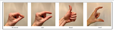
Therefore, subjective estimates of loudness are necessary. There are studies of categorical loudness scaling (CLS) in cochlear implant recipients [3] in which adult subjects participated. Results were reliable ones. What to do with children? We tried to use CLS for assessment of the loudness in cochlear implanted children. The aim of our study is how to find the equal loud C-levels in all channels and using these C-levels to create program with equal loud C-levels. Our study has a practical purpose, so we did not estimate the loudness function. We will not discuss the individual electrical levels of discomfort due to the large differences of these current values between listeners. The CLS is started when we had done reflexometry and parents selected an optimal program. We use our four pictures corresponding to categories “NO SOUND”, “SOFT”, “GOOD” and “LOUD” as a function of the electrical stimulus level (Figure 1).

Figure 1: Four categories of loudness

Lupinepublishers-openaccess-otolaryngology-journal

What reference electrical levels do we use?

Soft Levels

As we wrote earlier, at first day of fitting we approximately defined comfort levels (C-levels) which a child hears as quiet sounds [4].These stimulation levels had been recorded as C-levels in MAP3 of the first configuration. N.B. It is possible that the child did not hear a sound in some channels. Since by the time CLS starts, the child has some experience assessing the loudness of sounds, we can try to clarify these quiet C-levels. We use the first two pictures. This is a part of the CSL already. We stimulate, in our opinion, a quiet signal and “ask”. If child does not hear, we show picture “NO SOUND”. If child hears we show picture “SOFT”. Further, we reduce C-level below the threshold of hearing (2 presses on “Pg down”) and stimulate. We show squeezed fingers – “NO SOUND”. We repeat stimulation on different electrical levels involving the child in this game-study.

Loud Levels

By the time the CLS will be performed at relatively loud С-levels, we had done a reflexometry. How it is performed was described in our article [5]. N.B. In the case of absence of intraoperative ipsilateral reflex, it is impossible to exclude the presence of the contralateral reflex. We created a reflex-program with C-levels equal to the threshold levels of the reflex and recorded it as MAP2 of new configuration. It is known that different children can hear the different intensity of the sounds (from not too loud to loud) at the program where C-levels are equal to reflex threshold levels (our MAP 2). From this reflex-program we had created 3 programs and write them into the configuration. The first MAP is 3 steps lower, and 3-rd and 4-th maps are 3 and 6 steps louder correspondingly. In accordance with our instruction-explanation (“Program is optimal one if your child sometimes hears loud sounds” [6] speech therapists and parents selected optimal (working) program. It should be noted that almost all patients successfully use programs with C-levels above the reflex threshold levels by 3-6 steps (MAP3 and MAP4) [7] and even more. This is normal physiological phenomenon.

When we fit the patient without intraoperative reflex we work in accordance with the standard algorithm of fitting [8]. We gradually increase (in parallel) C-levels at all the electrodes until the parents and we’ll see that some program is loud one. Below this program is a working program (the optimal). Threshold levels are set to 10 percent of C-levels. Using this working program children respond well to all sounds and do not display negative reaction when surrounding sounds are the loud ones. Children can use a louder program in a quiet environment, but a child does not like it in a loud environment (according to parents’ comment). For the purposes of the CLS we use the test program, in which C-levels are less than levels of working program by 3 steps.

Why do we use a program less than optimal one for CLS? The child uses the optimal program in everyday life without problems, but when he will hear a sequence of long-term (300 ms) stimuli with an interval of 300 ms (SWEEP mode) on the one channel at maximal C-levels, the sensation can be unpleasant. N.B. Before CLS, it is necessary to visually assess the child’s reaction to the presentation of single and SWEEP stimuli at the C - levels of the test program - is there any negative reaction? Quite possible that child will not like the maximum C-levels of test program on some channels. C-levels in such channels must be corrected. Corrected C-levels of this test program will be used as loud sounds of the “LOUD” picture.

So. What do we have for our research?

A child hears and orients in sounds in accordance with an information of speech therapists and parents. Parents and teachers have identified a working program that the child uses without problems in all sound environments. Its C-levels are equal (very very rarely) or higher (almost all patients) than threshold levels of stapedial reflex. A child uses CI readily, in the morning the child asks to wear CI himself. A child indicates that the optimal program is the best one. (We asked parents to switch on processor at the first program –the child indicated to change the program). We know approximate loudness of some electrical levels. We know electrical levels, where the child hears quietly. We know where the child hears loudly - at C-levels of the test program. We know where the child hears well- in the area of the third quarter of the dynamic range of the audible current. The child has some experience of distinction between “SOFT” levels and “NO SOUND”. We can start the Categorical Loudness Scaling.

Methodics

How Do We Perform Categorical Loudness Scaling?

We use SWEEP stimulation, i.e. we provide a sequence of identical stimuli of the same amplitude on one channel. The duration of stimuli is 300 ms, the interval between them is 300 ms. SWEEP stimulation is started by pressing down the “Enter” button. The duration of the stimulation is determined by the duration of pressing the “Enter” key and the reaction of the child. We start CLS with a channel with a central frequency in the area of 800-1000Hz. We use categories “NO SOUND”, “SOFT”, “GOOD” and “LOUD” as a function of the electrical stimulus level. At first, we show our fig. 1 to the child. Child already has some experience in categories “NO SOUND” and SOFT”. We show signs with our fingers and explain what the volumes of the sound the child will hear in his (her) head (ear). Owing to our practice, we think that our pictures are more understandable and natural signs for description of child’s own sensation than a circle, squares, cubes etc. These signs are easier to repeat by children. Children may understand meaning of these signs from the birth.

We explain to the child that now we will stimulate, and he will hear a sound in the head (ear). We show the second picture, repeat the sign with our fingers and transmit quiet SWEEP-stimuli. We “ask” the child. If child agrees that he hears a quiet sound, we invite him to show it in the picture or with his fingers. Switching off stimulation, we squeeze fingers, show the first picture, that now there is no signal. Next, we show that we are going to increase the sound. We increase C-levels to 60% of the C-level of test program. We show the “GOOD” picture, raise our thumb and send SWEEP-stimuli. “Ask”. If child agrees, we invite him to show it in the picture or with his fingers. Switching off stimulation, we are clenching fingers, show that now there is no signal. The child agrees. Changing the electrical levels up-down we show with our fingers and on the corresponding picture how loud the signal or no signal will be heard. We invite him to show by his fingers or at appropriate picture. That’s how we perform the CLS training. After some training, a child begins to navigate in their feelings and to give real answers. When we reduce the level of stimulation the child brings own fingers closer, when we increase-move apart. Or they show the corresponding picture. He should be praised. Now we can go to the loudness estimations of the stimuli from the third quarter of the dynamic current range. When a child is assessing of the sound as “GOOD” we “ask” him if it is possible to increase the level of stimulus a little. Waiting for consent or refusal. Many children agree of our offer to slightly increase the stimulation. Then we increase C-level by 1-2 steps, stimulate and look how child displays this increase. Or by fingers, or on pictures. So, we move to the maximal C-levels of our test program where child will hear loudly i.e.to the fourth picture. Closely observe a behavior of the children during the CLS and involve them in the process!

It is curious to note that if some children show estimations of loudness not with their fingers, but with the pictures, they can show their ratings between pictures. For this reason, all four pictures must be placed in one line. Some children begin to show their estimations by the distance between palms. If the child is a contact one and cooperates with the audiologist, you can propose him to increase levels in order to gently touch the threshold discomfort levels. For this purpose, it is necessary to increase a C-levels of test program. But this is the best result. Repeated CLS measurements were done using single-electrode stimuli at a few electrode positions (sometimes all). C-levels at unmeasured electrodes were interpolated. The results were recorded. At the end of the CLS, we set equal-loud C-levels at all channels and make a program. Further, we compare these C-levels with the C-levels of working program defined by parents and teachers. We create new program with C-levels close to C-levels of working program. Since the C-levels of the created program and the working one are not the same ones, we check new program vootiue (on the child’s own ear) and create one program of 3 steps lower and 2 programs by 3 and 6 steps higher. Parents choose an optimal program in accordance with our instruction-explanation [8].

During the CLS we “communicate” with the child, “ask” and “explain”. Naturally, by signs: gestures, fingers, touching, facial expression and praise. We think that such a relationship is interesting to the child - child cooperates with the audiologist, we praise him for his work, correct mistakes, rejoices for the correct answer. Children tend to participate in this “research-game” with interest. We think that children are interested in judging the volume of sounds of different intensity and frequency, that’s why they willingly participate in the CLS.

Discussion

Children work in the CLS successfully. But loudness is a subjective evaluation. Naturally, for example, the same “LOUD” ratings of different patients will be different if they are measured in the terms of SPLs. We believe that the child himself chooses some criteria for assessing the loudness of sound and relies on it for all channels. It is quite natural for each patient to have his criterion, but we hope it is the same one for each child. Somehow it is used in repeated measurements on the different electrodes. Stable repeatable estimates are confirmation of this thesis. Every child adjusted all channels in accordance with own volume criterion. It is clear that adults also have their own criteria too, based on which they assess the loudness of the stimuli. But adult participants themselves noted difficulties in assessing the loudness of singlechannel stimuli of different spectral color. During the development of the fitting program SHCHUP [9] in which the stepped noises are used, adult patients themselves said that the estimation of the loudness of the stepped noises is easier than the loudness estimation of single-channel stimuli. Of course, children have the same difficulties. So, it is clear that the results of CLS on separate channels are not the completion of the fitting of children. The results of the detection equal loud(!) C-levels are important to configure the same equal loud levels in all channels and create a program. Despite the successful mastering of CLS by children, the last step of the fitting is the SHCHUP [9] . SHCHUP is the definition of comfortable SPLs of the stepped noises. The estimation of loudness of the stepped noises is a simpler task for experienced in CLS children too. On the base of SHCHUP’s results, we create four programs in new configuration.

The last step of fitting is the parents’ evaluation of the child’s perception of these programs in different sound environments and the definition of the optimal program in accordance with our instruction-explanation (Petrov & Tsjuk, 2015). Several hundred children (I did not count) participated in procedure of CLS, and I can surely say that the categorical loudness scaling in the fitting of cochlear implant children works successfully. We are sure that CLS is interesting game-procedure for the implanted children and useful method for an audiologist in order to fit children successfully. The CLS is a good encouraging and illustrative program for parents too. For example, we increased the level of stimuli and said mother that sound will be louder now. We stimulate and she sees that her child moves his fingers wider or moves his finger on the fig. 1 to the right. We reduce the level of stimulus and tell mother that sound will be quieter now. We stimulate and she sees that her child brings fingers closer or moves a finger on the fig. 1 to the left. At zero level, child squeezes his fingers together. So CLS is interesting and encouraging procedure for parents - mother sees the coherence of our words about changing of intensity (up or down) and the child response. Mothers are glad that her child correctly assesses the volume of sounds. This article describes General guidelines for performing of CLS. The main aim of this article is to guide how to teach the CI child to assess the loudness of sounds that is very important in the fitting process. Naturally, each child needs his own approach and this CLS, of course, is not done immediately. Speech therapists can use these pictures in their job with implanted patients and hard of hearing children too. Perhaps this method of the CLS can be patented.

Read More Lupine Publishers Otolaryngology Journal Articles:
https://lupine-publishers-otolaryngology.blogspot.com/

Saturday, 30 January 2021

Lupine Publishers | An Actual Statistical Problem with Model Selection My Solution

 Lupine Publishers | Journal of Otolaryngology


Introduction

This manuscript is a follow-up of my last one in SJO where I promised to show you my solution of a client problem. This case has been transformed such, that the logic of the problem remained unchanged and the confidentiality of my client’s data is warranted, however. In the last manuscript the results of the commonly found methods of modelling were shown and discussed. Now we will show my results and a discussion of them. Mathematically speaking the mainstream models already shown could be summarized as two univariate approximations by straight lines or a two-dimensional fit of a plane, describing the dependent variable by an approximation based simultaneously by a constant and two linear terms. I was fully aware of the limitations of the very small sample size of the mainstream models and I hope to successfully use this example to convince my readers about the economic benefits of discussions with professional mathematicians/statisticians instead of users of statistical software as I have classified them.

Methods

As I was blinded to the actual meaning of the variables X1, X2 and Y my experience indicated that I should try a second order polynomial fit as this would be the simplest possible model extension as compared to the mainstream linear models. The similarity to the considerations of Occam’s razor (see Wikipedia) are also well based on my personal professional experience. My model equation used is displayed below:

Y (X1; X2) =a0 + a1. X1 + a2. X2 + a3. X12 + a4. X1. X2 + a5 .X22 + error term (equ 1)

The above equation contains prior regression analysis the coefficients a0, a1 and a2 for the linear terms and a3, a4 and a5 for second order polynomial terms which must be estimated from the data by means of linear regression based on the method of least squares. The error term must fulfil the assumption that the data points represent statistically independent observations with constant variance in the domain of data points and an approximate Gaussian distribution. The most important data requirement is a continuous and metric measurement scale of the data and based on my long- term experience in medicine and other statistical applications, if fulfilled, the basis for a highly robust behavior of the regression analyses based on least squares. Finally, enough data points must be available. This is a problem in the determination of the sample size, which, in my opinion, requires professional statistical assessment.

Result

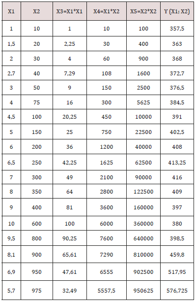
The numerical details are shown in Table 1 below with additional information necessary in the Excel data analysis software as the input for Excel’s regression routine:

a) Note 1: X1 and X2 and Y refer to the client provided original data. The author intended to look at a standard polynomial of degree 2 and the calculated data columns indicate all second order terms necessary from Excel logic for that purpose. The contents after the provided Y in the brackets are a help to understand that Y (as provided from my client) is the dependent variable of X1 and X2 in this very model. For physicians unfamiliar with exponential floating-point formatted numbers reading of the Excel online documentation is recommended.

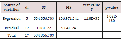
b) Note 2: There are three lines in Table 2. The descriptions in column one show regression in the first, residual in the second and total in the third line. The total in line 3 displays the SS of all data against the grand mean. The residual in line 2 shows the sum of squares of the differences between data and calculated Y values using the coefficients a0, a1, …, a5 and the line 1 described as regression provides us with the information of the explained variation by the calculated regression coefficients. In view of the raw Y data shown in Table 1 we observed therefore a residual variance - in the magnitude of 9,0403. 10-28 which – for practical purposes – might be judged as zero. The mathematical interpretation in everyday language is there is an interpolation problem or a perfect fit between the raw Y data and the regression equation with the calculated coefficients shown in

Table 1:

lupinepublishers-openaccess-otolaryngology-journal

Table 2: ANOVA analysis of variance table

lupinepublishers-openaccess-otolaryngology-journal

df: degrees of freedom

SS: sum of squares

MS: mean squares (represent the variances which are the squared

standard deviations).

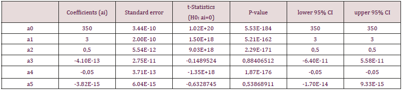
c) Note 3: The coefficients ai refer to the equation (1). Please note that i = 0, 1, 2, …, 5 in column one and a0 is frequently assigned the name intercept. We follow the frequently engaged standard statistical practice of setting not statistically significant coefficients to zero and have the solution of our model (from equation (1)) in equation (2) below:

Y (X1; X2) = 350 + 3. X1 + 0,5. X2 - 0,05. X1. X2 (equ 2)

The inevitable rounding errors which are present in all common computers are reflected in the Excel documentation which states that about ten to twelve digits in decimal results should be reliably exact. Therefore, it seems not to be a problem that 95% confidence intervals cover zero and actual numbers of digits of the raw data in Table 3 justify this decision. We analyzed in addition the model of equation 2 and for practical purposes we concluded that there were perfectly consistent results (data on file but not shown here). You might consider this fact as a simple way to be on the safe side with our conclusions about this data set. Our verbal comment to equation (2) is that the available data set very strongly indicates that a perfect functional relationship between X1, X2 and Y exists. In view of the relatively small sample size of the evaluated data here, it is strongly recommended to collect substantially larger data sets in the next future and only if results could be reproduced within the sampling error limits then an application for the Nobel Price could be envisaged in case our data originated from medical data.

Table 3:

lupinepublishers-openaccess-otolaryngology-journal

Conclusion/Discussion

The reader should consider several aspects of our example: First, finding practical interpolation from data sets could have apart from chances for a successful Nobel price application and small sample sizes other causes, e. g. that the Y-data is already a derived data item calculated from X1 and X2 actually. The originator of the data set could be consulted, and this issue might sometimes be clarified quickly. Second, a review of the selection criteria might shed additional aspects and one of the most likely finding might be that the data were collected from young, healthy volunteering soldiers instead of a larger sample with males and females in about 1:1 relation. Many other explanations for such a result might be presented here, but I think that an experienced statistician would likely be a valuable contributor to such – admittedly very rare – events. I think under all circumstances the plan for a follow-up study could be quite a challenge for the responsible physician as well. I’d like to emphasize that from a mathematical viewpoint a real and strong and simple functional relationship (interpolation) is likely to be considered as a very strong scientific revelation, finally. Another important consideration was in the results’ section mentioned and I’d like to address it here: In case of a polynomial of degree k with a sample n=k+1 there will be always an interpolation solution, which is just due to lack of sample size and as such not informative at all. My personal experience indicates very strongly that in cases where n-k coefficients are estimated and two k is at least contained in n-k several times then degenerate interpolation could safely be excluded, however.

In my early professional work life I was once confronted to a study to assess the effect of a substance on the blood pressure and heart rate which did not contain blood pressure as a selection criterion. It seemed to everybody as highly representative for the selected patients. Based on some 150 patients the baseline data showed certain, quite considerably big percentages of hypotonic, normotonic and hypertonic patients. The evaluation of baseline to end of treatment differences showed only a very weak linear trend for the changes of systolic, diastolic blood pressure and heart rate. A second order polynomial showed a clear, statistically highly significant quadratic trend: The hypotonic patients showed increased blood pressure data, normotonic had just data varying around zero and hypertonic patients showed statistically highly significant blood pressure reductions. Sponsor’s headquarter asked me to provide the average blood pressures from the full sample and as I assume - the international medical director - decided not to pursue this substance as the pooled average across hypotensive, normotensive and hypertensive patients was medically relatively small compared to the established hypertensive drugs of this pharmaceutical giant. It is no surprise at all, that a subgroup evaluation of the three blood pressure subgroups clearly indicated that young and middle-aged patients revealed quite small shares of hypertensive patients and patients aged over 60 years had considerable shares of hypertensive patients consistent with published literature of epidemiology. Today, I still judge this as a mistake based on the omnipresent linear thinking of the very company’s headquarter. Finally, I think the examples discussed here are at least some evidence that non-linearity can be present in medical data and the consequences could cause major detrimental damages to financial operations of corporations and by withholding potentially interesting drugs from patients’ unnecessary burden of disease(s).

Read More Lupine Publishers Otolaryngology Journal Articles:
https://lupine-publishers-otolaryngology.blogspot.com/

Friday, 22 January 2021

Lupine Publishers | Nasolabial Cyst: Report of 2 Cases and Literature Review

 Lupine Publishers | Journal of Otolaryngology


Abstract

Introduction: Nasolabial cysts are a rare, ectodermal development cyst, presenting as a fullness of canine fossa, nasal ala or vestibule of the nose. They are usually asymptomatic but may become infected. Treatment is complete surgical excision by sublabial approach, or transanal endoscopic marsupialization.

Case Report: Description of two cases, one female presenting as nasal deformity due to progressive growth of unilateral nasolabial cyst, and a healthy young male presenting severe facial cellulitis, with a CT showing bilateral nasolabial cysts.

Discussion: Nasolabial cyst is a rare condition, but diagnosis and treatment are simple. Nasolabial cyst should be incorporated by ENT in the differential diagnosis of nose deformities and facial swelling.

Introduction

Nasolabial cysts are also described as nasoalveolar cyst or Klestadt cyst and were first described by Zuckerkandl [1,2]. They are rare, affecting 1,6 per 100.000 persons per year, more frequently in females (4:1 ratio), especially among African Americans, in the fourth and fifth decades of life. 90% are unilateral, and often underdiagnosed [3,4]. Nasolabial cysts are non-odontogenic cysts that develop lateral to the midline of the maxillary lip and alar base. They usually present as a swelling in the nasolabial fold, causing alar nose elevation and upper lip projection. They may grow slowly and painlessly over several years. Because of its close anatomical relation to the nasal cavity and teeth, they may become infected easily, rapidly growing and being painful [1,5]. Diagnosis is made by clinical examination, imaging tests, and is confirmed by histopathologic study. The cyst can be palpated bimanually with one finger in the floor of the nasal vestibule and another in the labial sulcus. Computed tomography (CT) and magnetic resonance (MR) can be useful. Differential diagnosis includes cysts of the nasopalatine duct, periapical inflammatory lesions (granuloma cyst, abscess), and epidermoid cysts [1,6]. Complete surgical excision of the nasolabial cyst is the best treatment, and sublabial approach is most used. Other authors propose transanal marsupialization as an easier and shorter procedure, with lesser complications, but recurrence may be a problem [3,5].

Case Report 1

Figure 1(a).

lupinepublishers-openaccess-journal-otolaryngology

Y=372.256 + 6.8856. X1+residuals

52-year-old female patient with a 3-year history of left floor of nose intermittent painful swelling, and progressive deformity of this area. Computed tomography (CT) study showed a 3,2 cm rounded lesion in left pyriform aperture compatible with nasoalveolar cyst (Figure 1). A sublabial approach was performed, and complete excision of the cyst was obtained (Figure 2). Histological study confirmed suspected diagnosis. Patient evolved in excellent conditions, with no complications or recurrence in a 2 year follow up period.

Figure 1(b).

lupinepublishers-openaccess-journal-otolaryngology

Figure 1(c).

lupinepublishers-openaccess-journal-otolaryngology

Figure 2. Intraoperative view of sublabial access to left nasolabial cyst in Case 1.

lupinepublishers-openaccess-journal-otolaryngology

Case Report 2

Figure 3. Computed tomography of bilateral nasoalveolar cysts. Case 2.

lupinepublishers-openaccess-journal-otolaryngology

Figure 4. Pathology H-E study of Case 2 showing cyst wall with pseudostratified columnar cells.

lupinepublishers-openaccess-journal-otolaryngology

37-year-old male patient, with no prior medical record, developed a facial cellulitis with no initial response to oral antibiotics, requiring hospitalization and intravenous antibiotic treatment. Maxillary and orbital CT study showed bilateral nasoalveolar cysts, with signs of active infection in the right cyst (Figure 3). Antibiotic treatment was completed, and cyst resection was programmed a month later. An extensa sublabial approach was performed, and bilateral cysts were removed. Histological findings confirmed diagnosis (Figure 4). Patient did not have any other episode of facial cellulitis or cyst recurrence in a 14 month follow up

Discussion

Origin of nasolabial cysts is controversial. Most accepted theories are that cysts derive from remnants of the nasolacrimal duct or inclusion cysts of mesenchymal cells during the fusion of medial and lateral nasal prominences to the maxillary prominence during facial skeletal formation [2]. Histology usually present pseudostratified columnar epithelium. Su et al noticed with electronic microscopy that that cysts had a highly placated mucosa, of non-ciliated stratified columnar epithelium, differing from the ciliated columnar epithelium of the paranasal and nasal sinuses [7]. The treatment of nasolabial cysts consists on complete removal of the lesion, with the objective of prevention of infectious complications, histologic diagnosis, and aesthetic improvement. Fine needle aspiration can help in diagnosis, and relieve of symptoms, but recurrence is high [1]. Surgery is usually done by sublabial approach, creating a mucosal flap of gingiva to allow access to the pyriform aperture and to the cyst, which can be resected carefully to avoid rupture, especially to the floor of the nose mucosa, and complete excision is mandatory to avoid recurrence. After the intervention, the gingival mucosal flap is fixed in its original position with absorbable sutures. Potential complications are uncommon, including facial swelling, insensitive gingiva, teeth numbness, and surgical site infection.

Patients must use a toothbrush on the surgical site. Diet should be soft for the first week, then normal. Dental prostheses can be used immediately after surgery [1]. Lee et al published in 2009 a comparative study between surgical techniques, and strongly suggested endoscopic trans nasal marsupialization as a simpler, shorter and safer procedure, and in most cases, it could be done under local anesthesia [3]. In our two cases we used sublabial approach with general anesthesia because is the usual technique used in our practice, but we are interested to use endoscopic marsupialization in next cases. We did not have any complications or recurrences in follow up of both cases.

Conclusion

Nasolabial cysts are rare but must be considered in the differential diagnosis of floor of the nose deformities and facial swelling. Sublabial approach is the most common procedure, but probably be replaced by endoscopic marsupialization in the future.

Read More Lupine Publishers Otolaryngology Journal Articles:
https://lupine-publishers-otolaryngology.blogspot.com/

Thursday, 21 January 2021

Lupine Publishers | The Transfiguration with Self-Phase Modulation Effect of Entanglement in A Plasmatic Moving Frame

 Lupine Publishers | Journal of Otolaryngology


Abstract

In quantum optics, the Heisenberg picture, in which the optical fields can be treated as conjugate positions and momenta of quantized harmonic oscillators, as it is easy to substitute optical fields in classical electromagnetic problems with noncommutative operators and obtain the Heisenberg equations of motion. Once the operator equations are solved, it is possible obtain various quantum properties of the optical fields via noncommutative algebra. The Heisenberg picture is often not without shortcomings. Its difficulties have led to a growing appreciation of the Schrödinger picture, where the photons are treated as an ensemble of bosons and the evolution of the many-photon probability can be used. This is more intuitive approach that has led to great success in the quantum theory of solitons. Instead of solving the formidable nonlinear operator equations, we can obtain analytic solutions from the linear boson equations in plasmatic the Schrödinger picture which lead to the theory of Plasmatic Moving Frames.

Keywords: The Heisenberg Picture; The Optical Fields; The Plasma in Physics; Plasma in Medicine; The Many Photon Probability; Solitons, The Schrödinger Picture; Nonlinear Operator Equations; Plasmatic Moving Frame

Introduction

Plasma

(Figure 1) Plasma (from Ancient Greek πλάσμα, meaning ‘moldable substance [1]) is one of the four fundamental states of matter, and was first described by chemist Irving Langmuir [2] in the 1920s [3]. Plasma can be artificially generated by heating or subjecting a neutral gas to a strong electromagnetic field to the point where an ionized gaseous substance becomes increasingly electrically conductive, and long-range electromagnetic fields dominate the behaviour of the matter [4]. Plasma and ionized gases have properties and display behaviors unlike those of the other states, and the transition between them is mostly a matter of nomenclature [2] and subject to interpretation [5]. Based on the surrounding environmental temperature and density, partially ionized or fully ionized forms of plasma may be produced. Neon signs and lightning are examples of partially ionized plasma [6]. The Earth’s ionosphere is a plasma and the magnetosphere contains plasma in the Earth’s surrounding space environment. The interior of the Sun is an example of fully ionized plasma, [7] along with the solar corona [8] and stars [9]. Positive charges in ions are achieved by stripping away electrons orbiting the atomic nuclei, where the total number of electrons removed is related to either increasing temperature or the local density of other ionized matter. This also can be accompanied by the dissociation of molecular bonds, [10] though this process is distinctly different from chemical processes of ion interactions in liquids or the behaviour of shared ions in metals. The response of plasma to electromagnetic fields is used in many modern technological devices, such as plasma televisions or plasma etching [11]. Plasma may be the most abundant form of ordinary matter in the universe, [12] although this hypothesis is currently tentative based on the existence and unknown properties of dark matter. Plasma is mostly associated with stars, extending to the rarefied intracluster medium and possibly the intergalactic regions [13].

Definition

Plasma is a state of matter in which an ionized gaseous substance becomes highly electrically conductive to the point that long-range electric and magnetic fields dominate the behaviour of the matter. The plasma state can be contrasted with the other states: solid, liquid, and gas. Plasma is an electrically neutral medium of unbound positive and negative particles (i.e. the overall charge of a plasma is roughly zero). Although these particles are unbound, they are not “free” in the sense of not experiencing forces. Moving charged particles generate an electric current within a magnetic field, and any movement of a charged plasma particle affects and is affected by the fields created by the other charges. In turn this governs collective behaviour with many degrees of variation [10].

Figure 1: Top: Lightning and neon lights are commonplace generators of plasma. Bottom left: A plasma globe, illustrating some of the more complex plasma.

lupinepublishers-openaccess-journal-otolaryngology

Mathematical Descriptions

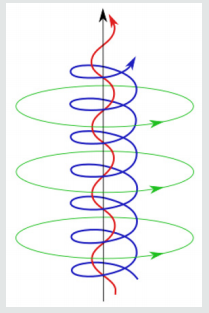
(Figure 2) The complex self-constricting magnetic field lines and current paths in a field aligned Birkeland current that can develop in a plasma. To completely describe the state of a plasma, all of the particle locations and velocities that describe the electromagnetic field in the plasma region would need to be written down. However, it is generally not practical or necessary to keep track of all the particles in a plasma. Therefore, plasma physicists commonly use less detailed descriptions, of which there are two main types:

Figure 2.
lupinepublishers-openaccess-journal-otolaryngology

a) Fluid Model

Fluid models describe plasmas in terms of smoothed quantities, like density and averaged velocity around each position (see Plasma parameters). One simple fluid model, magnetohydrodynamics, treats the plasma as a single fluid governed by a combination of Maxwell’s equations and the Navier–Stokes equations. A more general description is the two-fluid plasma picture, where the ions and electrons are described separately. Fluid models are often accurate when collisional is sufficiently high to keep the plasma velocity distribution close to a Maxwell–Boltzmann distribution. Because fluid models usually describe the plasma in terms of a single flow at a certain temperature at each spatial location, they can neither capture velocity space structures like beams or double layers, nor resolve wave-particle effects.

b) Kinetic Model

Kinetic models describe the particle velocity distribution function at each point in the plasma and therefore do not need to assume a Maxwell–Boltzmann distribution. A kinetic description is often necessary for collision less plasmas. There are two common approaches to kinetic description of a plasma. One is based on representing the smoothed distribution function on a grid in velocity and position. The other, known as the particle-in-cell (PIC) technique, includes kinetic information by following the trajectories of a large number of individual particles. Kinetic models are generally more computationally intensive than fluid models. The Vlasov equation may be used to describe the dynamics of a system of charged particles interacting with an electromagnetic field. In magnetized plasmas, a gyrokinetic approach can substantially reduce the computational expense of a fully kinetic simulation.

c) The spatiotemporal entanglement evolution in free space

The many-boson interpretation may be applied to study of entangled photons as well, where the two-photon probability is used to obey the Wolf equations by Saleh, Teich, and Sergijenko (STS). Instead of treating the entanglement properties of the photons, and the optical propagation as two separate problems, with the STS equations, we can use now a single quantity – namely, the two-photon amplitude – to keep track of the spatiotemporal entanglement evolution in free space. This is analogous to the Wolf equations, which reformulate the laws of optics in terms of coherence propagation. We utilize the STS treatment of the two photons in study of various temporal effects. The Schrödinger picture would offer a more accessible interpretation of temporal entanglement propagation for studies of two-photon systems. For example, a four-wave mixing in a coherently prepared atomic gas, thus extending the STS model for use in many more topics in quantum optics in order to demonstrate the use and intuitiveness of the Schrödinger picture. Based on this formalism, we propose the concept of quantum plasmatic temporal imaging, which uses dispersive elements and temporal phase modulators to manipulate the temporal entanglement properties of two photons. It is possible to convert positive-time correlation to negative-time correlation, or vice versa, using a plasmatic temporal imaging system.

This conversion technique could be immensely useful for applications that require negative-time correlation, such as quantum-enhanced clock synchronization. Generating of negativetime correlation directly has some shortcomings compared with the conventional tried-and-true schemes that generate positivetime correlation. This technique could allow more flexibility in choosing two-photon sources for quantum optics applications. We can consider two photons in two optical modes, such as two polarization, two propagation directions, or two waveguide modes. The two-photon wave function is

lupinepublishers-openaccess-journal-otolaryngology

Where the constants C s are overall amplitudes of the quantum states, is the quantum state in which one photon is in each mode, is the state in which both photons are in mode 1 and is the state in which both photons are in mode 2. The positive-frequency forwardpropagating component of the electric field in each mode is given by

lupinepublishers-openaccess-journal-otolaryngology

Where is the complex, frequency-dependent refractive index in mode , is the real part of , S is an area of quantization in the x-y plane, and is the photon annihilation operator, related to the corresponding creator operator via the equal-space commutator

lupinepublishers-openaccess-journal-otolaryngology

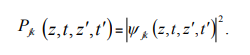
The physical significance of each amplitude is that its magnitude squared gives the probability density of coincidentally measuring one photon in mode j at (z,t) and another photon in mode k at ,

lupinepublishers-openaccess-journal-otolaryngology

Plasmatic temporal entanglement is defined as irreducibility of into a product of one-photon amplitudes in the form of a(t)b( ). This means that the probability of detecting a photon in mode 1 at time t is correlated to the probability of detecting a photon in mode 2 at . The most popular ways of generated entangled photons are spontaneous parametric down-conversion and four-wave mixing, where wave-mixing geometry and the spatiotemporal profile of the pump-beam determine the initial . (17, 18)

The most interesting case is when M=-1 and one of the photons is time reversed. If the two photons are initially entangled with positive-time correlation can be written as , where b is assumed to be much sharper than a. After photon 1 has passed through the plasmatic temporal imaging system M=-1 The photons hence become anticorrelated in time. Since most conventional two-photon sources generate positive-time correlation, but negative-time correlation is desirable for many applications, one can use the temporal imaging system to convert the former to the latter.


Besides the above application, one can also convert negativetime correlation, which can be generated by ultrashort pulses for improved efficiency, to positive correlation. Any desired correlation can actually be imposed on already entangled photons, by multiplying the original correlation with a factor of 1/M. As groupvelocity dispersion and temporal phase modulation play analogous roles in the time domain to diffraction and lenses, which can be use Fourier optics, temporal imaging, and quantum imaging techniques to design more complex quantum plasmatic temporal imaging systems. The quantum destructive interference via a coupler is determined by the overlap of the two photons amplitude with its plasmatic mirror image. The output amplitude is the destructive interference between the original amplitude and its replica but with the two photons exchanging their positions in time. In particular, for a 50%-50% coupler, T=R=1/2, complete destructive interference is produced if the two photons are temporarily indistinguishable. The introduction of variable distinguishability to photons, in order to produce varying degrees of destructive interference via a beam splitter to measure the two-coherence time, is the basic principle of the Hong-Ou-Mandel interferometer. As envisioned by Lukin and Imamoglu, the third-order nonlinear effects among two photons can become significant in a coherently prepared plasmatic atomic gas. The coupled-mode equations and then become nonlinear, where is the self-phase modulation coefficient and also cross-phase modulation coefficient. The advantage of the Schrödinger picture is most evident, whereas in the Heisenberg picture one needs to solve nonlinear coupled-mode operator equations, in the Schrödinger picture, one only needs to solve linear equations, which are similar to the configuration-space model applied to the quantum theory of solitons. The delta function couples the two subspaces, so entanglement can emerge from unentangled photons. A soliton formed by two photons in orthogonal polarizations exerting crossphase modulation on each other. Studies of two photons in the same mode under the self-phase modulation effect have been performed by entanglement, and cross-phase modulation offers the distinct possibility of entangling two photons in different modes.

Consider the case in which two polarizations have the same group-velocity dispersion, so that, and there is one photon in each polarization. The evolution equation for

lupinepublishers-openaccess-journal-otolaryngology

Defining time coordinates in a plasmatic moving frame.

lupinepublishers-openaccess-journal-otolaryngology

we obtain the following equation for :

lupinepublishers-openaccess-journal-otolaryngology

This equation is a simple linear Schrödinger equation, describing a two-dimensional “wave function” in a moving frame subject to a potential. To solve for

explicitly, we define new time coordinates
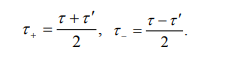
lupinepublishers-openaccess-journal-otolaryngology

The cross-phase modulation effect only offers confinement of along the time difference

axis, but not the mean arrival time axis. The only bound-state solution of is

lupinepublishers-openaccess-journal-otolaryngology

The delta potential enforces S to take on the value where and must have opposite signs.

For the final solution in the plasmatic moving frame of and is therefore

lupinepublishers-openaccess-journal-otolaryngology

The two-photon coherence time of a vector soliton is fixed, but he average arrival time is still subject to dispersive spreading and becomes increasingly uncertain as they propagate. Hence a two-photon vector soliton generates temporal entanglement with positive-time correlation as it propagates. Similar to the idea of soliton momentum squeezing, one can also abiotically change along the propagation axis to control independently the two-photon coherence time. The center frequencies of the photons are shifted slightly, by an amount of to compensate for their group-velocity mismatch, so they can copropagating at average group velocity. This is commonly known as soliton trapping. If the nonlinearity has a finite bandwidth, the potential becomes a finite-bandwidth function and multiple bound-state solutions can be obtained via conventional techniques of solving the linear the Schrödinger equation.

We have derived the general equations that govern the temporal evolution of two-photon probability amplitudes in different coupled optical modes. The formalism inspires the concept of quantum temporal imaging, which can manipulate the temporal entanglement of photons via conventional imaging techniques. The theory also offers an intuitive interpretation of two-photon entanglement evolution, as demonstrated by the exact solution of the two-photon vector soliton. To conclude, we expect the proposed formalism to be useful for many Plasmatic Moving Frames, quantum signal processing and communication applications.

Plasma Medicine

Plasma sources used in plasma medicine are typically “low temperature” plasma sources operated at atmospheric pressure. In this context, low temperature refers to temperatures similar to room temperature, usually slightly above. There is a strict upper limit of 50°C when treating tissue to avoid burns. The plasmas are only partially ionized, with less than 1 ppm of the gas being charged species, and the rest composed of neutral gas.

a) Dielectric-barrier discharges

Dielectric-barrier discharges are a type of plasma source that limits the current using a dielectric that covers one or both electrodes. A conventional DBD device comprises two planar electrodes with at least one of them covered with a dielectric material and the electrodes are separated by a small gap which is called the discharge gap. DBDs are usually driven by high AC voltages with frequencies in the kHz range. In order to use DC and 50/60 Hz power sources investigators developed the Resistive Barrier Discharge (RBD) [3]. However, for medical application of DBD devices, the human body itself can serve as one of the two electrodes making it sufficient to devise plasma sources that consist of only one electrode covered with a dielectric such as alumina or quartz. DBD for medical applications [4] such as for the inactivation of bacteria, [5] for treatment of skin diseases and wounds, tumor treatment [6] and disinfection of skin surface are currently under investigation. The treatment usually takes place in the room air. They are generally powered by several kilovolt biases using either AC or pulsed power supplies.

b) Atmospheric Pressure Plasma Jets

Atmospheric pressure plasma jets (APPJs) are a collection of plasma sources that use a gas flow to deliver the reactive species generated in the plasma to the tissue or sample. The gas used is usually helium or argon, sometimes with a small amount (< 5%) of O2, H2O or N2 mixed in to increase the production of chemically reactive atoms and molecules. The use of a noble gas keeps temperatures low and makes it simpler to produce a stable discharge. The gas flow also serves to generate a region where room air is in contact with and diffusing into the noble gas, which is where much of the reactive species are produced [7]. There is a large variety in jet designs used in experiments [8]. Many APPJs use a dielectric to limit current, just like in a DBD, but not all do. Those that use a dielectric to limit current usually consists of a tube made of quartz or alumina, with a high voltage electrode wrapped around the outside. There can also be a grounded electrode wrapped around the outside of the dielectric tube. Designs that do not use a dielectric to limit the current use a high voltage pin electrode at the center of the quartz tube. These devices all generate ionization waves that begin inside the jet and propagate out to mix with the ambient air. Even though the plasma may look continuous, it is actually a series of ionization waves or “plasma bullets”.(8) This ionization wave may or may not treat the tissue being treated. Direct contact of the plasma with the tissue or sample can result in dramatically larger amounts of reactive species, charged species, and photons being delivered to the sample [9]. One type of design that does not use a dielectric to limit the current is two planar electrodes with a gas flow running between them. In this case, the plasma does not exit the jet, and only the neutral atoms and molecules and photons reach the sample. Most devices of this type produce thin (mm diameter) plasma jets, larger surfaces can be treated simultaneously by joining many such jets or by multielectrode systems. Significantly larger surfaces can be treated than with an individual jet. Further, the distance between the device and the skin is to a certain degree variable, as the skin is not needed as a plasma electrode, significantly simplifying use on the patient. Low temperature plasma jets have been used in various biomedical applications ranging from the inactivation of bacteria to the killing of cancer cells [10].

Applications

Plasma medicine can be subdivided into three main fields:

a) Non-thermal atmospheric-pressure direct plasma for medical therapy.

b) Plasma-assisted modification of bio-relevant surfaces.

c) Plasma-based bio-decontamination and sterilization.

Non-thermal atmospheric-pressure plasma

One of challenges is the application of non-thermal plasmas directly on the surface of human body or on internal organs. Whereas for surface modification and biological decontamination both low-pressure and atmospheric pressure plasmas can be used, for direct therapeutic applications only atmospheric pressure plasma sources are applicable. The high reactivity of plasma is a result of different plasma components: electromagnetic radiation (UV/VUV, visible light, IR, high-frequency electromagnetic fields, etc.) on the one hand and ions, electrons and reactive chemical species, primarily radicals, on the other. Besides surgical plasma application like argon plasma coagulation (APC), [11] which is based on high-intensity lethal plasma effects, first and sporadic non-thermal therapeutic plasma applications are documented in literature [12]. However, the basic understanding of mechanisms of plasma effects on different components of living systems is in the early beginning. Especially for the field of direct therapeutic plasma application, a fundamental knowledge of the mechanisms of plasma interaction with living cells and tissue is essential as a scientific basis.

Mechanisms

Though many positive results have been seen in the experiments, it is not clear what the dominant mechanism of action is for any applications in plasma medicine. The plasma treatment generates reactive oxygen and nitrogen species, which include free radicals. These species include O, O3 , OH, H2 O2 , HO2 , NO, ONOOH and many others. This increase the oxidative stress on cells, which may explain the selective killing of cancer cells, which are already oxidatively stressed [13]. Additionally, prokaryotic cells may be more sensitive to the oxidative stress than eukaryotic cells, allowing for selective killing of bacteria.

It is known that electric fields can influence cell membranes from studies on electroporation. Electric fields on the cells being treated by a plasma jet can be high enough to produce electroporation, which may directly influence the cell behavior, or may simply allow more reactive species to enter the cell. Both physical and chemical properties of plasma are known to induce uptake of nanomaterials in cells. For example, the uptake of 20 nm gold nanoparticles can be stimulated in cancer cells using non-lethal doses of cold plasma. Uptake mechanisms involve both energy dependent endocytosis and energy independent transport across cell membranes [14]. The role of the immune system in plasma medicine has recently become very convincing. It is possible that the reactive species introduced by a plasma recruit a systemic immune response [15].

Conclusion

For the first time ever, physicists have captured an image of quantum entanglement. In a paper published in the journal of Scientific Advances, scientists from the University of Glasglow shared the first known image of a Bell entanglement. The photo depicts two photons interacting and sharing physical states for a brief instant -- an event that occurs regardless of the actual distance between the particles [16]. To capture a picture of the Bell entanglement, physicists created a system that shoots off streams of entangled photons from a quantum source of light at what they call “non-conventional objects.” These objects are displayed on liquidcrystal materials, which can change the phase of the photons as they move through them. A camera capable of detecting photons was then set to snap a photo when it identified one photon entangled with another. According to the researchers, quantum entanglement is one of the primary pillars of quantum mechanics. The concept is used in practical applications like quantum computing and cryptography, but no one has ever managed to capture an image of it in action. Physicists involved in the project believe that the image can help to advance the field of quantum computing and lead to new types of imaging [16-19]. These results confirm our theory on the Plasmatic Moving Frames (PMF).

The Transfiguration

As he was praying, the appearance of Jesus’s face changed, and his clothes became as bright as a flash of lightning [20]. While he was speaking, a cloud appeared and enveloped them, and they were afraid as they entered the cloud. (35) A voice came from the cloud, saying, “This is my Son, whom I have chosen; listen to him. LUKE 9: 29-36 These possible transfigurations is part of the abovementioned new types of imaging, what explanation and proves our theory of Plasmatic Moving Frames in quantum physics and optics.

Read More Lupine Publishers Otolaryngology Journal Articles:
https://lupine-publishers-otolaryngology.blogspot.com/