Showing posts with label soil and Environment Journals. Show all posts

Monday, 2 December 2019

Lupine Publishers | Spatial Analysis of Data on the Basis of the Digital Model of Relief and Locality (Example of Shemakha, Akhsu and Ismayilli Districts)

Abstract

The article examines the issues of studying the degree of susceptibility of sloping lands in Azerbaijan in the example of specific administrative territorial units, flat areas with a slope of up to 6% (about 3.50) are concentrated in Akhsu district 71%, and in Shemakha almost 49%. The steepest slopes are observed in the Ismaili region, where almost 26% of the territory has a slope of 10-18%, 30% of its area slope is 18%.


Introduction

Figure 1 Spatial analysis includes operations performed on geographic data using available methods and techniques in GIS software, with a view to describing the relationships between elements of the geographical environment. The analysis can be carried out on the data, both in the vector and raster systems, and touch the geometry and attributes of the vector data [1-8].
Figure 1.
lupinepublishers-openaccess-journal-environmental-soil-sciences

Search for Information in the Database

The main operation that can be performed based on the GIS database is information retrieval. This database has a relational nature and therefore, the object designation provokes the selection of the corresponding records from the corresponding attribute table, and vice versa. The first thematic layer in the database was the Digital Elevation Model in raster format. On its basis, as a result of the transformations and calculations, information on the height of the nos. and the slope of the terrain on the territory of Azerbaijan selected for analysis, which includes three regions: Shemakha, Akhsu and Ismayilli.

Vertical Position Factor

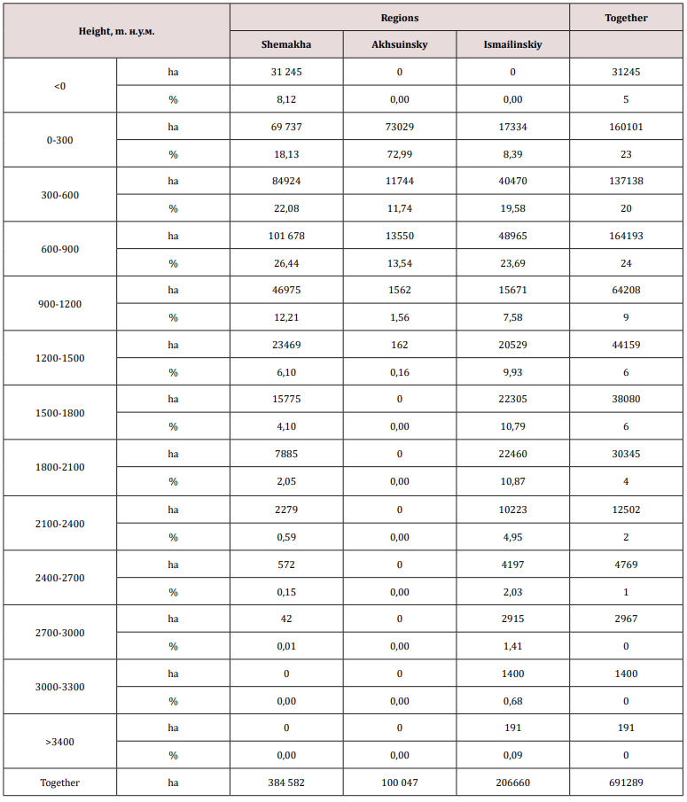
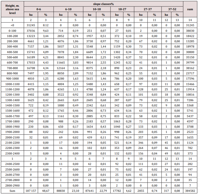
The major part of the study area is in the following ranges of heights: 1) from 0 to 300 mas-23.16%, from 300 to 600 m-19.84% and 3) 600-900 m-23, 75% of the total area. Above 900 m and up to 3400 m above sea level, about 30% of its area is located (Table 1). Of the administrative units belonging to the study area, the most highly allocated land Ismaili region. In this area 90: it is at an altitude of more than 300 meters above sea level, and sometimes the altitude is even higher than 3400 m. In Akhsu region about 73% of the earth is at an altitude up to the sea level. Shemakha district is an intermediate region, its largest area is at an altitude of 900 m above sea level-about 75%. In this area there is also a territory located below sea level-31244.66 hectares [8-18].

Classes of Slope

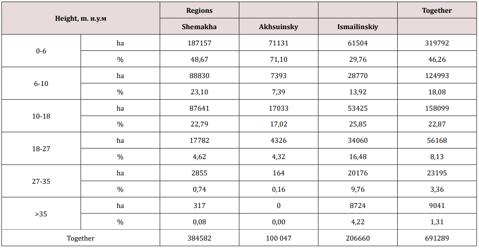
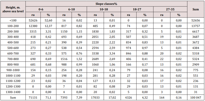
In the analyzed territory, the largest area is occupied by areas with a slope of up to 6-46%. Significant areas are also in the intervals from 6 to 10% -18% and from 18% to almost 23% of the total area (Table 2). Against the backdrop of administrative-territorial units, gently sloping areas with a slope of up to 6% (about 3.50) are concentrated in the Akhsu district 71%, and in Shemakha almost 49%. The steepest slopes are observed in the Ismaili region, where almost 26% of the territory has a slope of 10-18%, 30% of its area slope is 18%.
Table 1: The distribution of the study area (ha and%) over the altitude intervals.
lupinepublishers-openaccess-journal-environmental-soil-sciences
Table 2: The distribution of the study area (ha and%) over the slopes of the terrain.
lupinepublishers-openaccess-journal-environmental-soil-sciences

Classes of the Slope of the Terrain, Depending on the Altitude Intervals

Table 3: The distribution of the territory of the Shemakha district according to the grades of the terrain according to the altitude intervals.
lupinepublishers-openaccess-journal-environmental-soil-sciences
Table 4: Distribution of the territory of the Akhsu region according to the grade of the terrain depending on the altitude interval.
lupinepublishers-openaccess-journal-environmental-soil-sciences
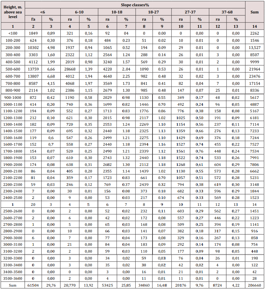
Table 5: The distribution of the territory of the Isma yilli region according to the grades of the terrain according to the altitude intervals.
lupinepublishers-openaccess-journal-environmental-soil-sciences
Tables 3-5 contain data that allow analyzing the distribution of the slope of the terrain along altitude intervals. This distribution was prepared for all administrative units of the area under consideration. In the Shemakha region, a clear dependence is shown, an increase in the slope, along with an increase in altitude above sea level. Up to a height of 1200 m there are lands with a slight slope-up to 6% (3.50). They occupy 49% of the area. Territories here with a slope of 6-10% and 10-18% are located at an altitude of 400-1700 m. M.u.m. about 23% of the area’s area. Areas with a slope of more than 18% make up more than 5% of the total area and are located in the highlands. In the Aksuinsky area, the terrain with an insignificant slope of up to 6% (3.50) prevails and they are located mainly at an altitude of 300 m above sea level - this is 71% of the total area. Areas with a slope of more than 6% are located at altitudes from 300 to 1400 m above sea level - about 29%. Clearly marked (17% of the total area) of land with a slope of 10-18% (6- 100) (Table 4).

In the Ismayilli region, most of the territory with a slope of &alt;6 to 10% is located at an altitude of 300 to 900 m above sea level. Areas with a slope of 10 to 37% occur at an altitude of 3000 meters above sea level. Locations with a slope of more than 37%% are located at the highest altitude but make up only 4% of the total area of the area. The second, from the thematic layers created in the database, is the land use of the study area. Due to the availability of cartographic materials, it was considered exclusively for the territory of the Akhsu district.

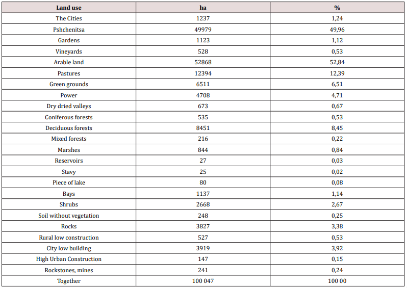
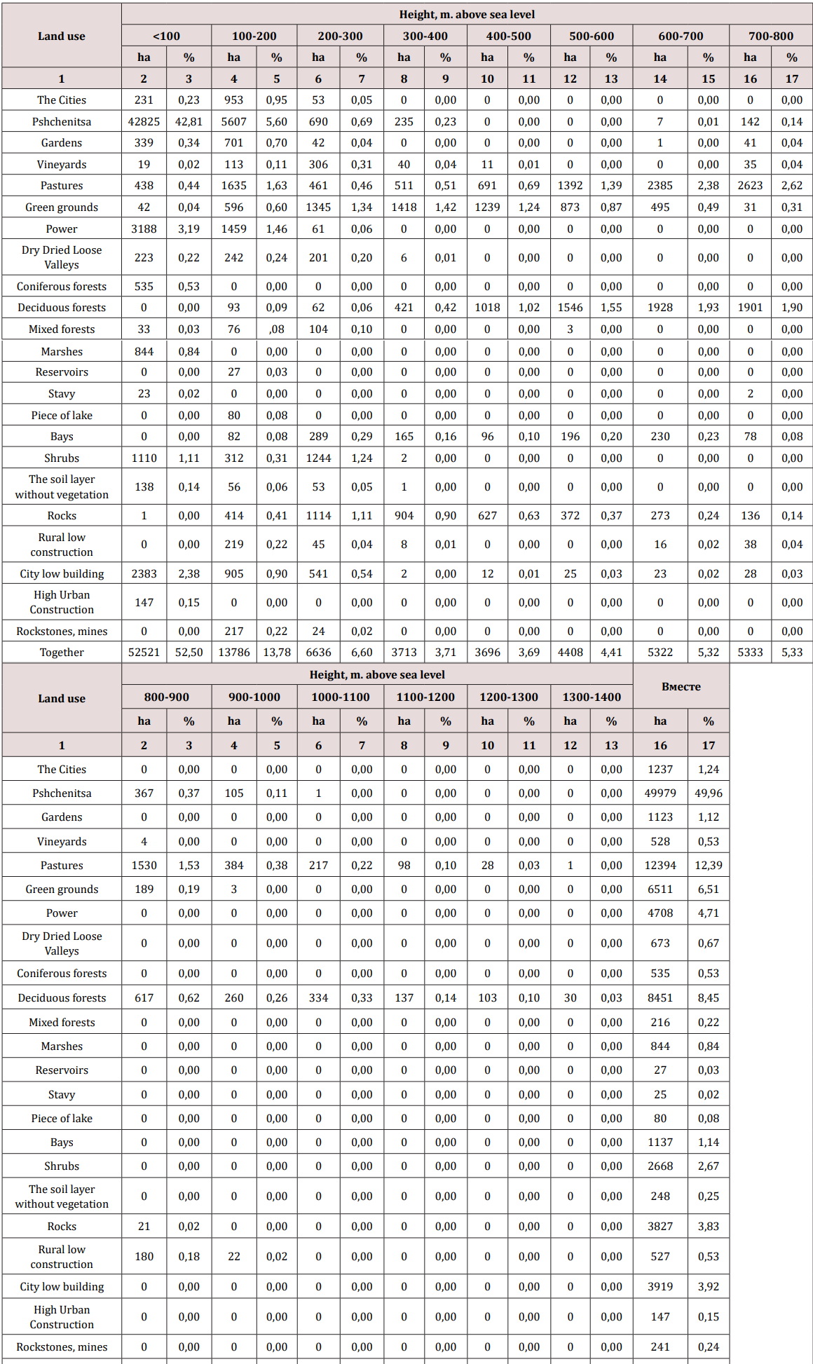
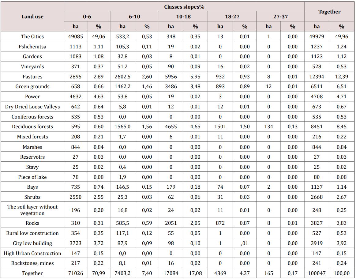
Analysis of the structure of land use in the Akhsu district showed that it is purely agricultural. The area is dominated by arable land, which makes up about 50% and tilled areas, which include pastures, meadows and degrees - more than 23% of the total area. Agricultural lands are supplemented with vegetable gardens, orchards and vineyards, occupying 3% of the area. There are few forests and shrubs, in general, about 12%. There are also areas completely devoid of vegetation in the Akhsu district, about 4% of them. A small part is occupied by water reservoirs, wetlands and urban and rural areas, amounting to 6.9% of the total area (Tables 6-8) provide information on the distribution of land use patterns over altitudinal intervals and grades of terrain slopes. Most agricultural land is located at a height of up to 400 m above sea level. Only pastures are located up to an altitude of 1400 meters above sea level. forest territories are in all altitude intervals. The remaining forms of land use are located at lower altitudes (Table 7). Considering the slope of the slopes, most of the territories are in the gradient class 0-6% - almost 71%. Only pastures, green lands, as well as deciduous forests, are located on slopes with a higher slope (Table 8).
Table 6: Land use in Ahsuinsky district.
lupinepublishers-openaccess-journal-environmental-soil-sciences
Table 7: Land use by altitude intervals.
lupinepublishers-openaccess-journal-environmental-soil-sciences
Table 8: Land use according to grades of the slope of the terrain.
lupinepublishers-openaccess-journal-environmental-soil-sciences


For more Lupine Publishers Open Access Journals Please visit our website:
For more Open Access Environment Journal articles Please Click Here:
To Know More About Open Access Publishers Please Click on Lupine Publishers

Wednesday, 20 November 2019

Lupine Publishers | Is the salvation of life on the planet?


Lupine Publishers- Environmental and Soil Science Journal


Before the advent of modern industry, nature had tangible additions in the composition of atmospheric water vapor natural evaporation from transpiration of plant and natural emissions, in particular, from the respiration of creatures, animal worlds. Every living being, every plant in its secretions, at the molecular level, in its secretions creates information about itself. It is known that in the exhalation of a living being in the moisture of breathing, in any secretions, information is contained. It is proved by the fact that animals determine their victims and the opposite sex by smells. Plants allocate their personal phytoncides. Phytoncides are all volatile substances released by plants, including those that are practically impossible to collect in appreciable amounts. These phytoncides are also called “native antimicrobial substances of plants http://stgetman.narod.ru/fitoncid.html. We all enjoy the smells of flowers, coniferous forests, shrubs.
Medicine has such achievements that it is possible to diagnose his illnesses according to the exhalation of a person. https://www. golos-ameriki.ru/a/254391.html The diagnosis of exhalation is the latest achievements of medicine, a revolution in oncology. Inspectors of road safety services for smell movement and appliances determine the state of alcohol status of the driver of the vehicle.All these smells and volatile substances are formed inside the living organism as a result of the most complicated chemical transformations. We also know that water has a different molecular structure and carries information. Maybe this information is preserved in evaporation? For example, in the works of the famous Japanese scientist Emoto Mazaru, it is clearly defined how ice crystals change depending on sound and even mental effects on water. Proceeding from this, it can be concluded that evaporation from organic matter also has certain properties and, accumulating in the atmosphere, creates certain conditions. It is these conditions that form the volumes of subsequent precipitation, the location of their distribution, and the graphs of precipitation.
A man with his civilization influences the path of organic transformations, or rather destroys a whole link in the everlasting path of water food chains. This is asphalt, arable land, surface water bodies, landfills. According to the area of the entire land area of the planet, such territories became 63 percent for 2015, which are expanding with the development of technologies with increasing acceleration. Even greater evaporation produces man from production and communal industries. Water coming from the water pipe evaporates in millions of evaporators, heaters, sinks, dryers from each rag, from each washed cup without changing the structure in the organics. These are evaporation unknown to the nature, let’s call them artificial.Nothing in nature is done just like that. Nothing never disappears anywhere and does not appear anywhere. What is the further path of artificial fumes? What is their structure, what is their volume and what is the speed of such evaporation. We feel it ourselves. They rise in the sky in huge volumes, they permanently cover the sun. They fall out incredible precipitation in some places, and do not carry drops into others. The mechanism of rational circulation has disappeared. This is no longer a cycle of water in nature, but a cycle of artificial fumes. Nature is powerless to control such volumes and such velocities.
It follows that organic evaporation, uniting in the clouds, synthesizes a certain substance, some special property that somehow forms the temperature, volume, shape, quality of the surface atmosphere. Interacting with the biota for millions of years, a certain cycle of substances between the atmosphere and the soil has stabilized. The quality, the amount of precipitation, the places of their condensation, movement in geographic space and loss all this was polished in a single process. This explains the creation and distribution of all natural areas from deserts to the tropics.From here we get droughts in some areas, floods in others. Destroyed, created by millions of years, the mechanism of atmospheric phenomena. In effect, the destruction of just one link in the circuit of water on the planet led to the creation of an entirely new atmospheric mechanism - the circulation of artificial fumes, a new source of natural disasters, to climate change.

Is There a Possibility of Salvation?

The Paris Agreements of 2015, “green technologies”, alternative energy sources - this is an intuitive direction created by mankind to conserve nature. Right direction. But only these are microscopic steps. Moreover, these steps lead to a catastrophe, diverting the efforts of mankind to preserve life.
The only true direction to preserving life on the planet is the movement to reduce artificial and return natural vapors. If we want to preserve life on the planet, we must begin to restore the nature of the cycle of water selected from it to nature.
A new concept for stopping climate change should be developed. The main elements of this are
a) Complete and unconditional stopping of projects and construction of all types of works with the partitioning of rivers, the laying of new channels
b) Global water saving in everyday life and production of all products by every person, every production of all countries and continents
c) Maximum possible rapid relocation of all types of production , the infrastructure of cities and the very housing under the ground.

For more Lupine Publishers Open Access Journals Please visit our website:
For more Open Access Environment Journal articles Please Click Here:
To Know More About Open Access Publishers Please Click on Lupine Publishers

Follow on Twitter   :  https://twitter.com/lupine_online


Tuesday, 19 November 2019

Lupine Publishers | Evaluation of Host Associated Genetic Markers for Rapid PCR Based Identification of Fecal Contamination Sources in Water


Lupine Publishers- Environmental and Soil Science Journal


Abstract

The water quality of many waterways in the state of Alabama, and in the nation as a whole, is deteriorating due to point and nonpoint source pollution from human and animal waste. Accurate identification of contamination sources is essential if we are to develop cost-effective pollution control strategies. The direct detection of host specific genetic markers by Polymerase Chain Reactions (PCR) has been widely used in identifying sources of fecal contamination in environmental waters. In this study, we conducted experiments to validate genetic markers associated with deer/elk, Canada goose, dog, and cattle for Microbial Source Tracking (MST) in Alabama. End point PCR was performed on 10 raw sewage samples and 133 fecal samples from nine animal species. Our results showed that CowM3, GFD (goose), and deer/elk associated markers have acceptable specificity and sensitivity, making them suitable for MST studies. However, the dog marker and one of the cattle markers (CowM2) exhibited cross reactions with other fecal samples. The performance of these host associated markers in environmental water was evaluated using both end point and quantitative PCR (qPCR). Human, goose, and dog markers were detected in several water samples by end point PCR; the human marker and CowM2 marker were also detected by qPCR. Samples collected after a significant rainfall event showed the highest frequency of genetic marker detection. Both human and Canada geese contributed to fecal pollution in samples from Parkerson Mill Creek.

Introduction

The water quality of many of the waterways in our state, and in the nation generally, is deteriorating due to contamination by both point and nonpoint source pollution from human and animal wastes. Each year, millions of cases of infectious disease result from swimming and bathing in contaminated water or consumption of shellfish harvested from fecal polluted waters [1]. Parkerson Mill Creek, located in east Alabama, is rated “impaired” because it fails to meet the water quality criteria required to support its designated use as a fish and wildlife stream. In 2007, the creek was included on the Alabama Department of Environmental Management’s (ADEM) 303(d) list of impaired waters for pathogens from point and nonpoint pollution sources. (http://adem.alabama.gov/programs/ water/303d.cnt). Urban runoff, pet waste, wildlife, and leaky sewer lines have all been thought to contribute to the high level of E. coli concentration (Parkerson Mill Creek Watershed Management Plan, 2010). However, more information is needed to definitively identify the major sources of fecal pollution in order to develop better strategies to protect against the health risks posed by polluted water. Fecal Indicator Bacteria (FIB) such as Escherichia coli ( E. coli) and Entero cocci have been used to indicate fecal pollution and potential human health risks in surface water for some time (USEPA, 1986). However, FIB methods are not specific to any fecal sources and require at least 24 h to obtain results [2,3]. It is also possible for E. coli and Entero cocci to survive and regrow in sediment after being released into the environment [4-6]. Given that the accurate identification of contamination sources is essential for developing cost effective pollution control strategies, increasing interest is now being directed towards the use of library and cultivation independent Microbial Source Tracking (MST) methods based on the polymerase chain reaction (PCR) technique that target host specific molecular markers. Combining MST methods with end point PCR and qPCR should provide results that reflect the most recent fecal pollution and identify the sources, thus enabling us to develop better pollution control strategies [7-9].
Members of the order Bacteroidales are considered promising fecal indicators with which to monitor microbial water quality due to their host specificity, broad geographic stability, and high abundance in the gastrointestinal tract of warm-blooded animals [10-17]. However, Acteroidales are not present in the feces of every individual member of a species and the concentrations may also vary from one to another [18] suggested that Bacteroides in gulls are scarce and the horizontal transfer of Bacteroides from humans to gulls is common. As a result, the avian markers used in the current study targeted bacteria namely Catellicoccus marimammalium. The objective of this study was therefore to evaluate host specific genetic markers associated with dogs, cattle, geese and deer that are likely to affect the local watershed. Environmental water samples collected from Parkerson Mill Creek were used to determine the performance of these markers in the field.


Materials and Methods

Sample Collection

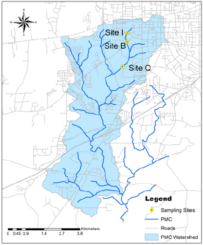
A total of 133 fecal samples and 10 wastewater samples were collected around three cities in east central Alabama, Auburn, Opelika, and Montgomery. The fecal specimens represented nine different animal species (cattle, Canada goose, cat, chicken, deer, dog, duck, goat, and horse) likely to affect the watersheds statewide and were collected with sterile wooden spatulas and placed in sterile polyethylene tubes. Ten raw human sewage samples were collected from nearby wastewater treatment plants in sterile 1-liter bottles. All samples were kept on ice and transported to the lab on the day of collection. Sewage samples were centrifuged at 5000 rpm at 4°C for 15 minutes to concentrate the solid materials 10-fold and fecal samples were stored at -80°C until use. On each of four days during the months of April and May in 2013 (April 12, 19, 26, and May 3rd), environmental water samples were collected from the surface of the water in three different sites in the Parkerson Mill Creek watershed (Figure1), a total of 12 samples were collected in sterile 1-liter plastic bottles. In order to extract the bacterial cells from the water, 500 ml of each sample was vacuum filtered through 0.45μm pore size, 47mm diameter nitrocellulose membrane filters (Thermo Fisher Scientific, Waltham, MA). The membrane filters were then stored at -20°C prior to DNA extraction.
Figure 1: Sampling sites in the Parkerson Mill Creek watershed.
lupinepublishers-openaccess-journal-environmental-soil-sciences

DNA Extraction

All DNA extractions were performed using the Power SoilTM DNA Isolation kit (Mo Bio Laboratories, Inc., Carlsbad, CA). Following the manufacturer’s instructions, 0.25 g of each fecal sample or 300μl of concentrated sewage were used for the DNA extraction. DNA from water samples were extracted from membrane filters that had been cut into small pieces prior to extraction. DNA concentrations were quantified using a NanoDrop ND-1000 UV spectrophotometer (Thermo Scientific, Wilmington, USA).

End-Point PCR and qPCR Assays

The primers used in this study are listed in Table 1. End-point PCRs were performed on a TGRADIENT thermal cycler (Whatman Biometra®, Germany). Each 25μl reaction mixture contained 5μl of 5x colorless GoTaq® Flexi buffer, 1.5mm of MgCl2 solution, 0.2 mM of dNTPs, 0.5μm each of the forward and reverse primers for the genetic markers, 0.4 mg/ml of bovine serum albumin (BSA), 0.08 unit/μl GoTaq® DNA polymerase, 2.0μl template DNA, and an appropriate volume of PCR grade water. The thermal cycling parameters for each PCR assay were 94°C for 2 min, followed by 30 cycles of 94°C 60s, 60°C (for the different markers’ annealing temperature please see (Table 1) 45 s, and 72°C 60 s, then 72°C for 7 min. The end-point PCR products were resolved using 1.5% agarose gel electrophorese and viewed under UV light to verify the absence or presence of the target gene. No Template Controls (NTC) containing PCR grade water only and positive controls were included in each instrument run for quality control. Real time PCR assays (All Bac, HF183, CowM3, and CowM2) were performed using the Step One real time PCR instrument (Applied Biosystems, NY). The reaction mixture (15μl) contained 1x SSO AdvancedTM SYBR® Green Super mix (BIO-RAD, CA), 0.7μg/μl BSA, 0.2μm of each primer and 5μl of template DNA. All reactions were performed in duplicate and began with a hold at 95°C for 10 min, followed by 40 cycles of 95°C 15s, 60°C 30 s, and 72°C 30 s. For each set of experiments, a no template control with two replicates was included and a calibration curve with a concentration spanning the range from 10 to 106 gene copies per reaction with two replicates was constructed.
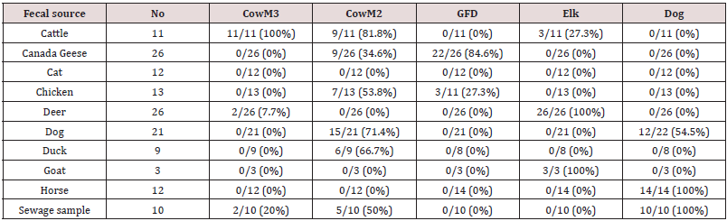
Table 1: Comparison of sensitivities and specificities of the host-associated genetic markers.
lupinepublishers-openaccess-journal-environmental-soil-sciences

Data Analysis

The Amplification Efficiencies (AE) were calculated based on the following equation:
E= 10(-1/slope) – 1
The related statistical analyses were performed using SAS® 9.3 software. ArcGIS 10.2 software for desk top was used to generate a sampling map for the Parkerson Mill Creek watershed.


Results

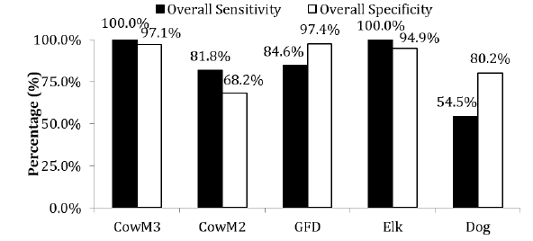
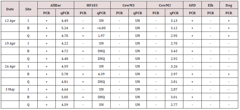
DNA extracts from a total of 133 fecal samples and 10 wastewater samples were analyzed and the results are shown in Table 1. The CowM3 Bacteroidales marker exhibited 100% sensitivity and 97.1% specificity, so the assay met the 80% benchmark suggested by the USEPA (2005) for both specificity and sensitivity. However, false positive amplification was also observed in four non-target DNA samples (two sewage and two deer samples). The CowM2 marker was present in 9 of 11 cattle fecal samples, resulting in 81.8% sensitivity. The CowM2 marker cross reacted with 42 non-target fecal DNA samples: 34.6% (n=9) Canada goose, 66.7% (n=6) duck, 50% (n=5) sewage, 71.4% (n=15) dog, and 53.8% (n=7) chicken, resulting in 68.2% specificity. Although the GFC marker for Canada goose was detected in 84.6% of the goose fecal samples it also exhibited a 100 % cross-reaction with human fecal samples, so in this case, we chose to use the GFD marker in our primer evaluation study instead. The GFD marker was positive in 84.6% and 27.3% of goose and chicken samples, respectively (Figure 2). The overall specificity and sensitivity of the GFD marker were 97.4% and 84.6%, respectively and although it had some cross reaction with chicken fecal samples (27.3%), it fully distinguished duck samples. Similarly, the elk marker was positive in 100% of the deer fecal samples, though it also cross reacted with the cattle (3/11) and goat (3/3) samples. The overall specificity and sensitivity of the elk marker were 94.9% and 100%, respectively. The dog marker was detected in 12 out of 22 dog fecal samples, 10 out of 10 sewage samples, and 14 out of 14 horse fecal samples, giving the dog marker the lowest values for specificity and sensitivity, at 80.2% and 54.5%, respectively, of the species tested. The All Bac genetic marker targeting the general Bacteroidales was detected in all 12 environmental water samples (Table 2). The human marker was detected in 6 out of 12 and 7 out of 12 water samples in the endpoint and real-time PCR assays, respectively. The Site B samples for all four sampling dates were positive for the human marker, as were the samples collected on April 12 and April 26 at site Q. Similarly, the dog marker was detected in one third (4 out of 12) of the water samples. The marker for Canada goose was detected in 58.3% (7 out of 12) of the water samples, with every sample from site B testing positive for this marker. Two samples from site Q, collected on April 12 and 26, showed positive results for the GFD marker. Neither CowM3 nor elk markers were detected in any of the 12 water samples.
Figure 2: Overall sensitivity and specificity of the different markers tested.
lupinepublishers-openaccess-journal-environmental-soil-sciences
Table 2: Detection of host associated genetic markers in water samples collected from Parkerson Mill Creek.
lupinepublishers-openaccess-journal-environmental-soil-sciences
(The unit for real-time PCR: log10 copies/100ml water).
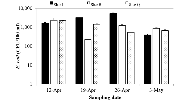
All of the 12 environmental water samples collected from the three locations were positive for E. coli (Figure 3), with concentrations ranging from 225 CFU/100 ml on April 19 at site B to 5200 CFU/100 ml on April 26 at site I. Both Site B and Site Q had significant high concentrations on April 12, probably due to the rainfall on that day. Site I had the largest geometric mean for E. coli concentration and site B the lowest. All sites exceeded the USEPA’s criterion for recreational water quality (USEPA 2012), which is a geometric mean of 126 CFU/100ml water. Eleven out of the 12 samples also exceeded the USEPA’s single sample maximum for E. coli concentration, which is 410 CFU/100ml. The relationship between the E. coli concentration and the All Bac marker concentration was weak (results didn’t show).
Figure 3: E. coli concentrations at all sampling locations for different dates (CFU/100ml).
lupinepublishers-openaccess-journal-environmental-soil-sciences

Discussion

The Canada goose specific genetic markers (GFC and GFD) were chosen for evaluation in our study. The other genetic markers used in our study to identify the sources of fecal pollution were based on Bacteroidales and its relatives (Table 1), as the order of Bacteroidales is known to be both abundant and common in mammalian feces. However [19] characterized the fecal microbial community from Canada goose, suggesting that the majority of the genes sequenced were related to Clostridia or Bacilli or, to a lesser degree, Bacteroidetes. Canada goose Bacteroidales specific genetic markers have also been reported elsewhere [20], but these genetic markers were not chosen for the current study because although they are relatively temporally stable, they have low sensitivities. In Green [18] study, the GFC and GFD markers targeted were Catellicoccus marimammalium and Helicobater spp., respectively, with GFC occurring at a higher concentration as more ribosomal operons in Catelli coccus.. However, the GFC marker failed to distinguish between waste pollution from human and goose samples in the present study, so we discontinued our evaluation of the GFC marker on other fecal samples. This result suggests that genetic markers need to be validated across a range of conditions, even when they appear to be highly specific when initially reported. Here, the GFD marker exhibited a 27.3% cross amplification with chicken samples, which is consistent with Green et al.’s research as GFD was originally developed to detect avian fecal samples. We found that it actually had a higher sensitivity (84.6%) on goose samples than the 68% reported in Green et al.’s original study. Therefore, our results for the GFD marker support the sensitivity and specificity of PCR assays for identifying Canada goose-associated fecal pollution in freshwater. CowM2 and CowM3 are both well-developed cattle associated Bacteroidales genetic markers that have been widely used in various MST research studies. Although CowM2 was reported to perform better than CowM3 by Raith et al. [21], a lower sensitivity for CowM2 (50%) has also been reported elsewhere [22]. However, the applicability of those results to other regions is potentially limited due to factors such as host diet, climate and geographic location. In our study, we found a much lower specificity for CowM2 (68.2%) compared with previous studies, some of which have reported values of over 98% [21,23,24]. There are several possible reasons for this discrepancy. First, geographical differences could affect host associated Bacteroidales markers significantly due to differences in the diet and animal digestive tract physiology. Layton [17] found that Bacteroidales 16S rRNA gene sequences obtained from pig were more closely related to Bacteroidales 16S rRNA gene sequences obtained from humans than to cattle sources, even though pig and cattle are in the same order of Artiodactyla. Second, the evaluation of the same set of samples may produce different results when examined from a presence absence or quantitative perspective. When there are cross reactions with non-target feces in PCR assays, this is usually at a low level compared with the signal for the target feces and will thus tend to be classified as false positives in end point PCR evaluations but not in real time PCR evaluations [25]. Third, the decay rates for the host-associated markers in the environment may be different due to their size and function [26]. CowM2 targets a 437 bp fragment as encoding an HDIG domain protein involved in energy metabolism and electron transport, while CowM3 targets a 569 bp fragment encoding a sialic acid-specific 9-O-acetylesterase secretory protein involving cell envelope biosynthesis and the degradation of surface polysaccharides and lipopolysaccharides [27-28], so the decay rate of these two proteins in environmental water after release from local animal tracts or the abundance variation of the proteins in fecal samples may explain the discrepancy.
The CowM3 marker, on the other hand, had an overall specificity of 97.1 % and 100% sensitivity, which is consistent with previous studies that reported CowM3 to have both a broader target host distribution and greater stability [21,27]. The relative abundance of the host associated genetic markers for CowM3 was 32.6 times greater than the CowM2 marker concentration in the same DNA sample, and this value compares favorably with the results previously reported by Shanks [28]. The amount of target gene in each cell may explain the different target copies detected in the same DNA samples by the different markers [29] pointed out that the CowM2 marker targets a single copy gene involved in energy metabolism. Here we hypothesize that there may be two or more CowM3 target genes involved in cell envelope biosynthesis and the degradation of surface polysaccharides and lipopolysaccharides. This result also indicates that not only is CowM3 more specific, but it also has higher sensitivity and a lower detection limit than CowM2 due to its greater abundance. Thus, it will be necessary to validate the specific genetic marker that will be used in each different geographic location because the performance characteristics may change and will thus affect the evaluation results. The dog associated marker DF475F was paired with Bacteroidales specific Bac708R and analyzed in our study against 143 target and non-target DNA samples. Dick [30] who developed this dog marker, found no cross amplifications with human, cat, cow, pig, chicken, or gull sources. However, they also pointed out that the horizontal transfer of fecal bacteria may occur among species in close contact, such as humans and their pets, which suggests the potential for cross reactions with the dog marker in human samples. This is probably why our results showed that this primer set amplified 100% of the sewage DNA representing human sources. Since this primer was the first and only dog specific primer that has yet been identified, the similar results for dog primer in Dick et al.’s research suggests the need for future work in this area to optimize the primer and reaction. Elk primer was found to amplify both the cattle and goat samples, which is consistent with previous studies that reported that deer/ elk primer could not distinguish between Bacteroidales sequences from deer/elk and sheep. Our results suggest that combining the results from CowM2, CowM3, and elk markers should make it possible to distinguish between cattle and deer/elk fecal pollution.

The All Bac genetic marker was designed to target the 16S rRNA genes of Bacteroides spp. and provides a rapid direct measurement of fecal contamination in water due to feces from warm-blooded animal sources [16]. The positive results for the All Bac genetic marker in all the water samples in the present study provides an estimate of the total fecal contamination present in the water samples. The human marker was detected in 6/12 and 7/12 of the water samples using end point and real time PCR assays, respectively. All samples from site B has been detected with HF183 marker, which suggests a potential source of human fecal pollution close to this sampling site. However, there was no CowM3 signal detected by either end-point PCR or real-time PCR. The discrepancy results were observed between end-point and real time PCR assays with CowM2 marker probably due to the cross-reaction of CowM2 marker with non-target feces since the low target concentration was detected. Given the lack of signal detected for the deer/elk marker, the positive signal for CowM2 in the environmental water samples is probably due to the presence of human fecal pollution. The samples that were positive for human signals also amplified the dog marker; these sites were Site B and Site Q on April 12, and Site B on April 26. Since the dog marker was detected in 100% of the human samples, the positive signal for the dog marker in the water samples was probably due to the presence of human fecal pollution. Similar results for the GFD marker are likely to indicate the presence of fecal pollution from Canada goose; during the sampling season, Canada geese were observed around the sampling site, which is consistent with these results. Interestingly, there was no signal detected due to the CowM3 marker in samples collected from site Q, even though this site is close to the beef teaching center at Auburn University and beef cattle were observed on site. That was probably because site Q was located at the upstream of beef teaching center. Future work may be needed to add more sampling sites locate downstream of beef teaching center. This result suggests the capacity of MST to identify major pollution sources from among many possible sources.


For more Lupine Publishers Open Access Journals Please visit our website:
For more Open Access Environment Journal articles Please Click Here:
To Know More About Open Access Publishers Please Click on Lupine Publishers

Follow on Twitter   :  https://twitter.com/lupine_online

Thursday, 7 November 2019

Lupine Publishers | The Study of Parameters and Reliability of Low-intensity Irrigation in the Conditions of Azerbaijan


Lupine Publishers- Environmental and Soil Science Journal


Introduction

In recent years, both in the Republic and in the CIS and far abroad are developing low-intensity stationary systems of irrigation, consisting of Micro Sprinklers, impulsive actions, aerosol auto oscillatory action sprinkling irrigation, auto oscillatory action auto oscillatory action combined, the drip, drip pulsing and a number of others. This is because low irrigation system has a number of significant advantages over other methods of irrigation. Especially promising the creation of automated sprinkling systems impulse machines, combined, auto oscillatory action stepper auto oscillatory action rocker type, pulse-airborne apparatus auto oscillatory action, etc. It should be noted that these systems allow to reduce the capital cost of their construction, also ensure the principle as “sprinkling” or “drip” in condition of daily water use plants. That is to create optimal conditions for the growth and development of plants during their growing season (Figure 1).
Figure 1:
lupinepublishers-openaccess-journal-environmental-soil-sciences


Moves the study

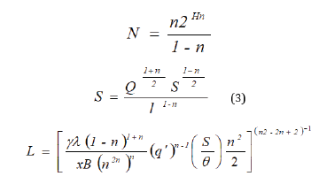
Automated watering crops the basis for high yields and productivity. Therefore, from the elements and devices used automatics require reliable and uninterrupted operation. Therefore, starting from the design stage through these devices and the production and operation, reliability issues, because the problem of reliability is not only technical, but also an important economic task. Reliability theory developed in recent decades, offers a great opportunity for a qualitative assessment of the reliability of existing irrigation technique, including micro irrigation systems. Reliabilitythis property of equipment or system to perform specified functions to maintain their performance within the required period or time required. From among the existing irrigation technique, stationary sprinkling system consisting of a large number of similar elements in a specific order on the field and required for the irrigation of crops. Determining the reliability of one of these elements will decide the reliability of systems. Reliability issues fixed irrigation systems in particular, equipped with sprinkling installations engaged in many of the scientists in the former Soviet Union and abroad. To examine the elements of the calculation on reliability of low-intensity sprinkling (for example pulse sprinkling auto oscillatory action) should consider the technological feasibility and sprinkler systems. Optimal low irrigation system parameters were determined by us by searching for the specific functions listed minimum cost with UD. Depending on the area of the system S; aspect ratio θ; the cost of the system (Q); Mr pressure corresponding to the pressure dictating point; conditional irrigation period tat equal i/q 3600 ì where, m irrigation norm, m; q / -maximum ordinate hydro-module m/s).
Number of distribution pipelines (N); the distance between irrigation technique (sprinkle plants) l; x factor, equal with the placement of devices on square 0.2; the length of the i-th pipeline system l(i) its diameter (D)(i) and discharge Q(i) , the coefficients (k), (m), β -dependent roughness of the internal the surface of the pipes; costs of irrigation Engineering (sprinkler devices, etc.). With g and the pressure Sn site; the cost of one kW/h of electricity; ψ, coefficient η pump unit equal to 0.7 coefficient of non-uniformity of flow
lupinepublishers-openaccess-journal-environmental-soil-sciences
gde, r- ratio splash start P2 to pressure end splash r1), equal to 1.02-1.25; factor e0 = e1 +e2 (e1, e2 -regulatory factors of efficiency of capital investments and annual deductions for depreciation and repairs); coefficients (b), (d) dependent on the material and the cost of pipe laying and operating costs of the attendants e(n): [1,2]
lupinepublishers-openaccess-journal-environmental-soil-sciences
Studies have shown that the most economical option is the simultaneous operation of all sprinkler devices system, i.e., when the system is produced by the limit dispersal of current irrigation [3] in this case has a minimum at points determined by the expressions:
lupinepublishers-openaccess-journal-environmental-soil-sciences
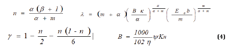
Where is
lupinepublishers-openaccess-journal-environmental-soil-sciences
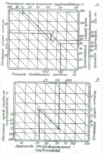
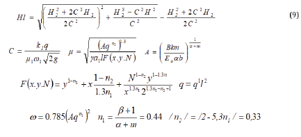
Substituting in the formula (3) and (4) coefficients corresponding to steel pipelines (d = 1.4; m = 5.1; β= 1.8; K = 0.00107; In = 50; E0 = 0.2; Ton = 1.1), obtain payment formula to determine and that for ease of use, represented by nomogram (Figure 2). Similar monograms built and for pipes made of plastics and other materials. Optimal pipeline diameters (D)opt, I, number of irrigation pipelines x, suspended from the distribution pipeline, number of sprinkler devices on the polynom pipeline y define the following ratios:
lupinepublishers-openaccess-journal-environmental-soil-sciences
Figure 2:
lupinepublishers-openaccess-journal-environmental-soil-sciences
If you change the original parameters S, q/, θ, m) within: < = 30 S < = 300 ha, 10 0.3-7 < = q/ < = 1.0 x 10⁻⁷ m/s, < 0.25 = θ < = 4, 0.3 < = M < = 1.0 m
1000 m3/HA, the optimal system settings change within: 35 < = l < = 135 m; 3 < = N < = 65; 1 = < x < = 50; and 1 < = y< = 33. Being attached to squares, laid down specific natural-economic conditions define systems parameters of irrigation on low-intensity pulsed example sprinkling [4]. Consider these square set and equal to 150- 400 ha and have an average optimal relationship of the parties 1-3 and natural-economic conditions irrigation norm 0.35-0.75 m and a maximum ordinate 0.6 x 10 hydro-module-7 -1.0 x 10⁻⁷ m/s.
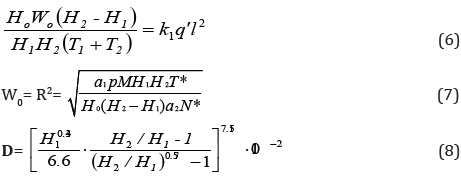
Averaged source data S= 200 ha, θ = 2; M = 0.55 m, q/ = 0.8 x-7 m/s, the following optimal system settings l= 50m, N= 22, x = 10, y = 8 obtained using the following programs and formulas (4.5). For other crops and natural-economic conditions these parameters are defined similarly. Obtained values of N, l, x, y, (D) opt. I -enable you to define the basic construction and technological parameters of irrigation equipment (impulse sprinklers apparatus self-oscillating action): as head n2, corresponding pressure start splash RV2, head n1, the pressure end splash r1; constructive volume pneumatic accumulator W0 and nozzle diameter (D) [3,5]. Based on the submissions of works of scientists of the world, and the results of Erosion and irrigation in the Institute research on some definition NANA parameters of irrigation technology in conventional machines, sprinkler machines pulse actions, etc., for which we offer the following characteristic control to determine the basic parameters of pulse devices depending on pressure. But corresponding to the initial pressure pneumatic accumulator p0 and the corresponding atmospheric pressure p and cross -sectional areas, bringing the pipeline ω2 inlet flow coefficients pneumatic accumulator μ1 and μ nozzles2, resources pneumatic accumulator t*, sprinkler apparatus N*, the coefficients that depend on the value of sprinkler apparatus (d)1 and (d)2, [1,2,3,7].
lupinepublishers-openaccess-journal-environmental-soil-sciences
It should be noted that equation (6) matches the water supply and water plants, and equation (7) and (8), respectively, the optimum size of sprinkler devices and agro technical requirements and quality of rain (the number of sprinklers drops with a diameter of more than 1.0-1.5 mm in overall flow rain Jet should be less than 10%). Each group of m, q, S, θ correspond definite values x, y, N, l and system settings h2 n1, W0, D pulse settings of the apparatus. Bearing in mind that the real system tM1 = t >M2 and sum of hydraulic resistance to worst according to the terms of the pnevmogidroakkumljatora filling system Σ ξ = > 1, equation (6) you can submit in the form: [1,7]
lupinepublishers-openaccess-journal-environmental-soil-sciences
Qi-factor of 2.64 for steel pipes. 10-3/Equation (7,8 and 9) together with the formula for Ap Ruseckogo represent a closed system of equations. The below Figure 2 provides a graphical solution of this system. Knowing the economic radius of action impulse apparatus and setting from system (= 3-5), the search for a solution should lead to corresponding with curves in the following order and1 and4, and7 and10 for s = 3, by and 2 and5 and8 and11 when c =4 and3 and6 and9 and12 when c =5. Parameters of sprinkler unit with intermediate values with determined by interpolation. Using the results obtained previously, define the structural and technological parameters of pulse apparatus for the same natural-economic conditions. With the placement of devices on the squares economy its radius R= 21-35, and c = 3 [1,3]. Using monographs s and the input values to and (C) pulse parameters are as follows:
(P)1= 450 kPa, P2 = 700 kPa, W0 = 0.19 m3, D= 20 mm.
To address the complex of actions on system reliability is reliability elements sprinkler systems. Research of reliability indicators of basic elements of fixed sprinkler system are the results of theoretical and experimental research, evaluated, tele control devices noise immunity parameters dispersion, irrigation norms precipitate individual sprinkling and installed types and parameters of distributions of operating time to failure of the main elements of the systems sprinkling [3,4]. In moments the adoption of tele control device command “select object” in the network of technological pipelines occur transients. Found that the pressure p can be set to lower static pressure reconfiguring tele control devices r/ 0 and duration of exposure of the false signal can reach 0.15-1.2 sec. Received the following experimentally confirmed the dependence between team processing time signal tk , swing Rod h effective membrane area (F)e, a cross section of tube connecting the technological pipeline with working hydraulic factor ω dental rigidity to the recoil spring2 , specific gravity γ water b and the acceleration of gravity (g) :
lupinepublishers-openaccess-journal-environmental-soil-sciences
According to the formula (10) evaluated the time reconfiguring device automated tele control. At instant slide. pressure in the hydraulic drive to atmospheric pressure, kPa, corresponding pressure 340 item Chooser requires 0.34 c 1.5 times greater than the duration of a false signal. (10) allows you to not only assess the time reconfiguring devices of automated process control systems tele control channel irrigation, but to appoint him constructive value parameters in accordance with the requirements of noise items tele control systems [3]
Start pressure dissipation of impulsive actions self-oscillatory apparatuses splash leads to dispersion of their volumes Δ splash W layer and therefore rain m, so how are they related dependencies.
(the number of cycles of performance in a year and its service area). Testing of pulse (100 picks) and the subsequent processing of the received data found that distribution of r2 and r1, subject to the normal law with coefficients of variation of νP2 = 0.04 and νP1 = 0.093. Bearing in mind
A what
the density distribution of m can be represented as:
lupinepublishers-openaccess-journal-environmental-soil-sciences
from constructive impulse imperfections. Obviously, the smaller the ratio δΔw/Δ W , the machine better.
Table 1:
lupinepublishers-openaccess-journal-environmental-soil-sciences
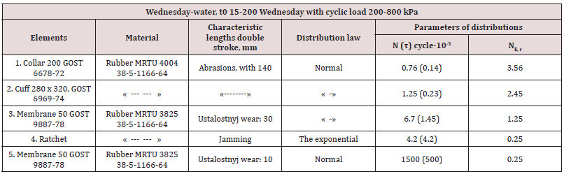
Studies (Table 1) on the definition of the types and distributions of operating time to failure ( N , σ- coverage and root mean square deviation) typical sprinkling systems devices, including the most common elements in hydro automatics: the underground sliding hydrants (elements 1, 2), devices, systems automated supervisory control (items 3, 4), yaw (element 5) as well as impulse sprinkler machines (6.7 items, 8, 9). It is established that the distribution of time to restore those elements, you can characterize the average recovery time tin [3,6].


Discussion of research results

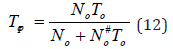
As a result of special research received the following relationship between the average service life of parts made of rubber or plastic tWed, the average number of cycles N# 0 a year and experimental aging value of these materials in the water t0equal to 6.8 years:
lupinepublishers-openaccess-journal-environmental-soil-sciences
In addition to these activities required to address the optimal level of operational reliability of stationary systems should develop institutional arrangements. For organizational activities of particular importance was the implementation of preventive works and correctly spent time. The timing of prevention is one of the main problems of preventive maintenance, which is closely linked to the content of preventive works and the Organization of their execution [7]. These terms are usually defined in the study the following objective function:
lupinepublishers-openaccess-journal-environmental-soil-sciences
where, with1,2 respectively, the cost of replacement of parts when troubleshooting failures and preventive replacements; (M) (t), N(t)-respectively, the average number of replacements in case of failure and preventive services for time t.


Scientific conclusions

Expelled us measure perfection is appropriate with a view to selecting the best design because it is economically summarizing indicators of maintainability of systems security, persistence, and sprinkling

For more Lupine Publishers Open Access Journals Please visit our website:
For more Open Access Environment Journal articles Please Click Here:
To Know More About Open Access Publishers Please Click on Lupine Publishers

Follow on Twitter   :  https://twitter.com/lupine_online

Thursday, 31 October 2019

Lupine Publishers | Response of Sandy Soil Stabilized by Polymer Additives


Lupine Publishers- Environmental and Soil Science Journal


Abstract

Traditional sandy soil stabilizers such as lime cement, fly ash and bituminous materials, etc., usually require long curing time. Hence now a day, polymer stabilizer is used more extensively because of its stable chemical property and shorter curing time. For the developing organization, it is important to judge the performance of stabilized soil during its developing stages only. This paper aims to highlight a quick and easy test to evaluate the mechanical performance of such polymer based stabilized soil. For this study, three different kinds of polymer stabilizers at developing stage were evaluated against a market ready product. The analysis of the test result include a comparison of the strength, moisture loss rate and strain energy under different curing time, polymer type, polymer additive amount and test conditions. This study shows that the strength of the stabilized sandy soil is significantly increased both under wet and dry conditions by using the polymer additives. With the procedure mentioned in the paper it was easier to identify the relative merits and demerits of each product.

Introduction

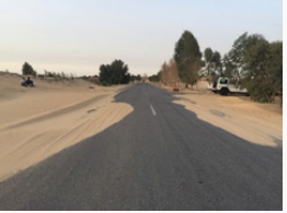
In the desert areas, large amount of soil is lifted by wind, the road is covered by the soil as shown in Figure 1, therefore, soil stabilization is important for road capacity. Soil stabilization is the alteration of one or more soil properties, by mechanical or chemical means, in order to maximize the suitability of soil for a given construction purpose by improving in-situ soil properties. Soils may be stabilized to increase engineering properties like strength and durability; or to diminish erosion and dust generation. The stabilized product should not only enhance desired soil properties, but they should also create a soil material/soil system which can sustain for the design life of the project, under designated load application. In the field application, the polymer dilution is sprayed normally into the loose soil. After polymer dilution penetrates into the soil, compaction of the “wet” soil is carried out. The stabilized soil gains strength after water evaporates from its soil mix. Traditional stabilization of soil relies on cement, lime, fly ash, and bituminous [1-3] material. As the scientists and researchers are developing new engineering materials, many non-traditional materials are available for soil stabilization, for examples polymer emulsion, acids, enzymes and tree resin emulsions [4-7]. As compared to the traditional stabilizers, these stabilizers have the following advantages:
Figure 1: Road covered by sand.
lupinepublishers-openaccess-journal-environmental-soil-sciences
a) Stable chemical properties;
b) They produce less swelling and heaving [8,9];
c) Produce less pollution; and
d) They save natural resources.
Apart from above mentioned benefits another advantage is that the liquid concentrate can be diluted with water and thus it is easy to achieve target additive amount by controlling dilution ratio. In many countries, large percentages of roads and parking lots are unpaved. The vehicles and wind together with the loose soil create dust that are known for adverse environmental and human health impact. Apart from increasing the strength of the soil these stabilizers can also be used as a way for controlling dust. For the ease of transportation and storage these Polymer emulsions can also be prepared in the form of powder. Before field application it is important for the industries to understand the mechanical properties of stabilized soil primarily during development phase of the product. Thus, the main objective of this paper is to highlight a quick and easy way to evaluate the mechanical performance of such stabilized soil before actual field application. Such assessment will quickly provide them a guide to modify their product if at all needed. For a comparison study, three in development products from the same company namely a) L13126; b) L13140; c) L13142 and one a market ready “Product A” is chosen, all as anonymous reference products. Overall, they constitute three polymer emulsions and one polymer powder type as described later in the paper. Goals within the scope of this paper include the following:
a) In detail description of sample preparation
b) To evaluate the property and suitability of the sandy soil before the addition of stabilizer developed by chemical polymerization techniques
c) To evaluate the property and suitability of the sandy soil after the addition of the stabilizer
d) To investigate the influence of the mechanical properties of the sandy soil with the polymer emulsion (in terms of mix proportion, percentage of stabilizing additive, water content and permeability of the stabilized soil matrix)
e) To demonstrate the influence of the emulsion types, curing time and wetting condition on the mechanical response of the stabilized soils
f) At last, present a relative ranking of various soil stabilizer products
The outcome of the tests is analyzed in terms of unconfined compressive (UC) tests. It is hereby noted that other tests such as California Bearing Ratio (CBR) [10,11], triaxial (confined and unconfined), resilient modulus, and cyclic wet dry tests are also valid tests to investigate the performance of the stabilized soils. However, for a rapid screening of stabilizers, the UC test was preferred. In this investigation, the compacted stabilized sandy soil samples were ‘cured’ under controlled temperature and humidity conditions before the soaked and un soaked unconfined compressive strength (UCS) tests were performed.

Material and Method

Materials Used

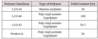
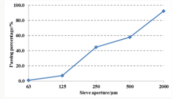
Four different kinds of stabilizers were used in this study, three polymer emulsion type namely: L13126, L13142 and Product A and one powder polymer type namely: L13140. Table 1 lists the polymer type and solid content of individual emulsion type, which was obtained by drying a known weight of emulsion in the oven at 1050C to a fixed weight. The sandy soil samples which contain 10% china clay and 90 % sand were considered which more or less represent a dust prone unpaved soil road. The sand used in this research is natural sand in Netherland, the gradation is showed in Figure 2.
Table 1: Polymer stabilizer type and polymer solid content
lupinepublishers-openaccess-journal-environmental-soil-sciences
Figure 2: Sieving test result of natural sand.
lupinepublishers-openaccess-journal-environmental-soil-sciences

Specimens Preparation

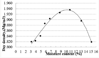
In order to perform compression tests, cylindrical specimens of 100 mm diameter and 150 mm height were prepared. The optimum moisture content of the sandy soil without stabilizer was measured by the modified proctor method (ASTM D1557). Figure 3 shows the result of modified proctor test. From the plot of the Figure 3, it can be observed that the optimum moisture content of this sandy soil is about 10.3%. With the known optimum moisture content and the known maximum dry density of the sandy soil, gyratory compactor was utilized (at 600kPa vertical stress, 30 gyrations/ min and 1.250 tilt angle) for the preparation of specimens. In order to mix the polymer stabilizer and soil uniformly, the stabilizer concentrate was diluted in the water before putting it into the sandy soil mixture. The dilution ratio was based upon the optimum moisture content and the amount of stabilizer used. For providing enough space for the polymer concentrate in the soil matrix, the stabilizer amount and the amount of water to be added is calculated on the basis of the optimum moisture content i.e. 10.3%. The actual density of polymer emulsion was assumed to be 1Kg/L. The preparation of sample was carried out in following six steps: soil preparation, additive preparation, soil-additive mixing, moulding, compaction, curing. The soil was mixed for five minutes before the addition of dilution. The amounts of added stabilizer were 14L/m3 (i.e. 1 m3 compacted soil contains 14L stabilizer concentrate), 19L/ m3 and 24L/m3 respectively. The dilution ratio was calculated by the following equation:
Figure 3: Modified proctor test result.
lupinepublishers-openaccess-journal-environmental-soil-sciences
where: R: dilution ratio
x: optimum water content (%)
y: maximum dry density of soil (Mg/m3)
z: amount of adding polymer (L/m3)
ρ: the density of stabilizer in the test temperature (Mg/L)
Assuming the depth of penetration in pavement to be 15 cm, the amount of addition of stabilizer i.e. 14L/m3, 19L/m3, 24L/m3 is equivalent to 2.1L/m2, 2.85L/m2, 3.6L/m2 respectively. After the soil and additive preparation steps, the dilution was mixed with sandy soil by using rotary mixer, until a uniform mixture was achieved. The specimen was prepared by using a gyratory compactor mould of 102 mm diameter and 254 mm height. The material was placed in three layers in the mold and each layer was compacted with rod for 25 times in order to get a uniform specimen. After molding step, the sample was placed in the gyratory device and compacted until the height of the sample was reduced to 150 mm. The compacted sample was then extruded from the gyratory mould by the hydraulic jack extrusion device mounted on the gyratory machine. The compacted sample was then placed in the curing room at 200C and 40 percent relative humidity. In order to simulate the field condition, air-dried curing process was used. Each sample was weighed after 3 days, 7 days, 14 days, 21 days, and 28 days to get the moisture loss rate.

Unconfined Compression Test

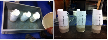
The sandy soil samples stabilized with the different type and number of additives were tested by using unconfined compression (UC) setup under soaked and un soaked conditions. In the soaked UC test, the dry sample was placed in the 25 mm deep water bath for 15 minutes and after removing it from the water it was drained for 5 minutes. Then the soaked samples, as shown in Figure 4, were tested. The soaked UC test reflects the influence of moisture on the strength reduction of the stabilized soil in the field condition.
Figure 4: Samples soaked in the water bath.
lupinepublishers-openaccess-journal-environmental-soil-sciences

Permeability Test

Permeability test was conducted to evaluate the capability of the stabilized soil samples to allow the water pass through it. The falling water head setup, see, is used for measuring permeability of the sandy soil samples with different types and amounts of the additives. In this test a sample is connected to a standpipe which provides both the water head and the means of measuring the quantity of water flowing through the sample. The permeability value is calculating by using the following formula:
Where: Kt: permeability(m/s)
a: cross section area of used manometer tube (cm2)
A: cross section area of sample in permeameter cell (cm2)
t: measured time interval (s)
L: length of sample (cm)
h1: start level manometer tube distance above overflow level (cm)
h2: end level manometer tube distance above overflow level (cm)
The parameters a, A, L were calculated on the basis of geometry of the samples and the manometer tube. The test was carried out after the sample was fully saturated. After that, the water tube is filled to a prescribed starting level h1. After t seconds, the water head level 2 in the manometer tube is recorded. By using the equation mentioned above the permeability Kt is calculated. The procedure is repeated at least three times interval until the Kt value is constant.

Results and Discussion

Optimal Polymer Adding Amount

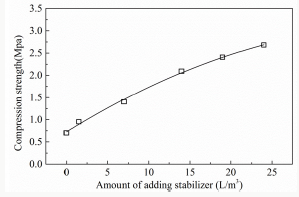
Preliminary test was conducted to get a reasonable amount of stabilizer quantity to be investigated, L13126 polymer was taken as an example, various additive amounts of 0L/m3 (pure water), 1.5L/ m3, 7L/m3, 14L/m3, 19L/m3 and 24L/m3 stabilizer quantity were examined. Figure 5 shows a plot of the additive amount versus UCS results after 28 days curing. As shown in Figure 5, the compression strength increases with stabilizer adding amount, it is expected that higher polymer content leads to thicker polymer matrix and more interaction between the soil particles, the compression strength increase almost linearly. It is hereby defined that “incremental strength” means the UCS of stabilized sample deducted by the UCS of samples with pure water. According to the Netherlands specification, the minimum UCS of bounded base layer shall be not less than 2MPa. Therefore, in this investigation, the incremental UCS value of 2 MPa was set as our minimum strength requirement. As can be seen from the prediction curve of Figure 5, the stabilized soil with 19L/m3 additive amount can reach 2 MPa. Therefore, the additive amount around 19L/m3 i.e. 14L/m3 and 24L/m3 and at 19L/m3 were investigated in the new test plan for all the polymer stabilizers.
Figure 5: Preliminary UCS test results.
lupinepublishers-openaccess-journal-environmental-soil-sciences

Polymer Adding Amount Effect

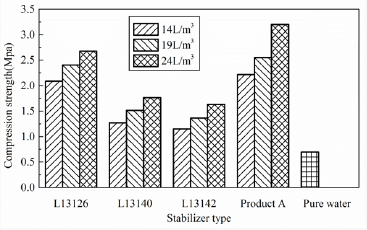
Figure 6 presents the UCS of sandy soil sample stabilized with different type and different adding amount after 28 days curing period. All the stabilized sandy soil demonstrated remarkable increase in UCS than the sample mixed with only pure water. The highest UCS value after 28 days curing period was found for Product A stabilized sandy soil which was higher than the sample stabilized by L13126. The L13140 and L13142 stabilized sandy soil show almost similar UCS values. However, as compared to the L13126 and Product A, these two stabilizers display lower UCS values. It is also noted hereby that UCS value increased with the increase in the stabilizer adding amount.
Figure 6: UCS values after 28 days curing.
lupinepublishers-openaccess-journal-environmental-soil-sciences

Wet and Dry Condition Effect

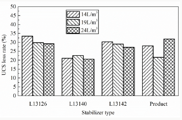
The soaked UCS of the sandy soil samples with pure water were not able to be tested because the samples disaggregated in the water bath. For comparison of moisture sensitivity of the samples, the strength loss rate of different stabilized samples was determined as Figure 7 In general, it can be observed that the strength loss rate decreases with the increase in the stabilizers amount, it indicates the thicker polymer coating will prevent moisture diffusion better. L13140 powder polymer specimens provide better water resistance to moisture deterioration and lose about 20% compression strength, the compression strength loss rate of others stabilizer specimens is about 30%. The specimens without stabilizer begin to disintegrate when they are placed in the water, and then lose load bearing capacity, the polymer can improve the water resistance of sandy soil.
Figure 7: UCS soaked loss rate after 28 curing days.
lupinepublishers-openaccess-journal-environmental-soil-sciences

Curing Time and moisture lose effect

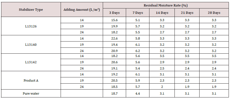
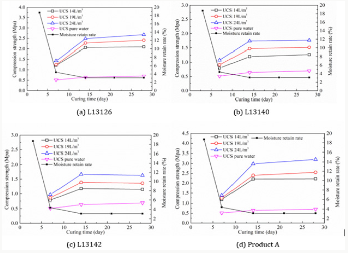
The effect of curing time on residual moisture rate is presented in Table 2, the value is based on the original water adding weight and the water loss weight. The samples were weighted after 3, 7, 14, 21 and 28 curing days, as shown in Table 2, the residual moisture rate became a constant, almost all the moisture has evaporated by the 14th day of curing for all the stabilizer specimens with different adding amount, the final value is not zero duo to the moisture loss in the mixture process. Comparing the values of specimens with stabilizer and pure water, the different is slight, it illustrates polymer do not affect the moisture evaporation. The moisture evaporates from the sample that will enhance the bonding between polymer and soil particles, the relation between compression strength and residual moisture rate are shown in Figure 8, duo to residual moisture rate decrease with curing time for all the specimens is similar, for brevity, the residual moisture rate result of pure water sample is taken as an example to compare with the compression strength variation. The sample with polymer stabilizers develop approximately 60% of the 28 days compression strength within the first 7 days of curing, however, the strength growth after 14 days curing period is not significant, the strength growth trend is similar to that of residual moisture rate decrease, this indicates that the gain in strength of the stabilized sample may only be related to the rate of moisture evaporation and not to any chemical reaction as normally observed in cementitious stabilized products.
Figure 8: Effect of curing time on compression strength.
lupinepublishers-openaccess-journal-environmental-soil-sciences
Table 2: Residual moisture rate.
lupinepublishers-openaccess-journal-environmental-soil-sciences
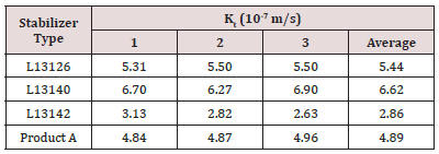
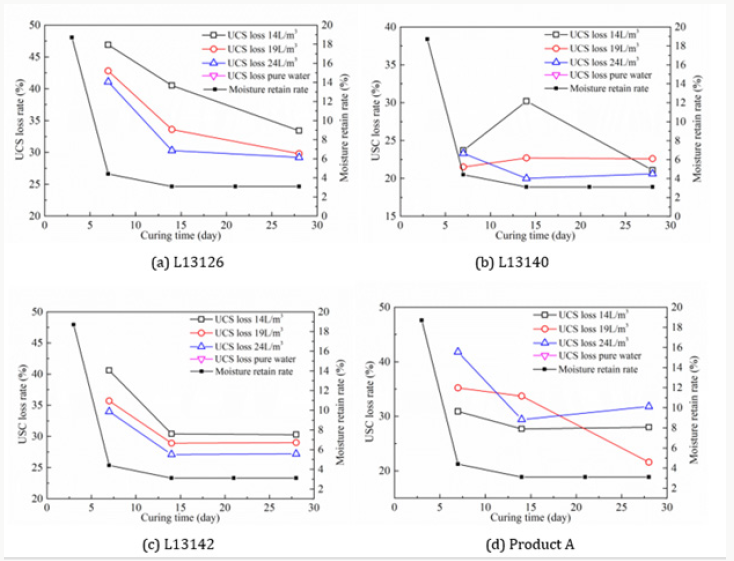
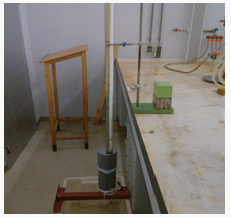
The moisture in the stabilized sample will influence the soaked UCS loss rate, the effect of curing time on USC loss rate is shown in Figure 9. In general, the USC loss rate decrease with the increase of curing time, the trend is similar to that of strength growth, it illustrates the sample with less moisture inside has a better moisture damage resistance. Samples utilized for permeability test were prepared in the same method as the ones used in the UC test (refer to “Specimens preparation” section). As shown in Figure 10, sample is kept inside the tube with no side flow allowed and the bottom 2 cm of the sample is utilized to apply silicon glue. After filling up the tube with water the test equipment is left for one day to be able to fully saturate the sample. The permeability test was carried out on the samples stabilized by L13126, L13140, L13142 and Product A with 19L/m3 additive amount, 3 replicates for each case, the permeability results are presented in the Table 3. It can be observed that all the sandy soil samples stabilized by the polymer stabilizers show lower permeability which is important for pavement surface layer to prevent rain water infiltration into the deeper part of the road foundation, soil stabilized by L13142 show highest permeability.
Figure 9: Effect of curing time on USC loss rate.
lupinepublishers-openaccess-journal-environmental-soil-sciences
Figure 10: Permeability test equipment.
lupinepublishers-openaccess-journal-environmental-soil-sciences
Table 3: Permeability test results.
lupinepublishers-openaccess-journal-environmental-soil-sciences

Implication and Discussion

Polymer is an environmental way for dust control and soil stabilization, as important as dust control, the mechanical and hydraulic property are also key points of polymer application, in this paper, mechanical and hydraulic property include three key indexes: UCS, soaked UCS loss rate and permeability, after 28 curing days, the moisture evaporate from the stabilized soil, the specimens become stronger and have a lower UCS loss rate. Unfortunately, there are no significant relation between the three indexes for all the polymers, the highest UCS is product A, the lowest UCS loss rate is L13140, and the lowest permeability is L13142, therefore it is hard to find a polymer with higher UCS, lower UCS loss rate and lower permeability, for the application, field condition, strength requirement and cost should be considered for stabilizer selection.

Conclusion

This paper in detail describes a quick and easy way, from sample preparation stage to experimental tests, to evaluate the performances of four kinds of stabilizers on sandy soil. With the results obtained from the tests one can examine the relative performances of various stabilizers. Such tests can be performed during product development phase itself. For example, from all the samples examined, tests results indicated that soil stabilized by L13126 has higher UCS both in soaked and un soaked conditions than the one stabilized by L13140 and L13142 and it is comparable to market ready Product A. The 28 days UCS of sandy soil samples stabilized by using 19L/m3 of L13126 and Product A can reach to a desired value of 2 Mpa (as per recommendation). Sandy soil stabilized by polymer powder L13140 is slightly stronger than the one stabilized by the polymer emulsion L13142. Such information can be used in the ranking of various products. Other findings that can be drawn from the results presented in this paper are summarized as follows.
a) This study shows that the strength of the stabilized sandy soil is significantly increased both under wet and dry conditions by using the polymer additives.
b) The UCS values of the sandy soil samples demonstrate that the polymer-stabilized soil properties improve with the curing conditions and the additive amount.
c) The increase in strength is observed due to the deposition of the solidified polymer components after water evaporates from the emulsion. The amount of polymer deposited on the surface of the soil particle depends on the concentration of the polymer and to the degree of mixing.
d) The compressive strength growth rate of the stabilized soil correlates with the moisture loss rate in the sample. There is no further strength increase when sample completely loses its moisture.
e) After 14 days, most stabilized soil samples reach the maximum compressive strength.
f) As compared to the cement & lime stabilized soil in literature, the stabilized soil sample shows higher deformability.
g) Sandy soil sample stabilized by the polymer stabilizers show lower permeability.

For more Lupine Publishers Open Access Journals Please visit our website:
For more Open Access Environment Journal articles Please Click Here:
To Know More About Open Access Publishers Please Click on Lupine Publishers

Follow on Twitter   :  https://twitter.com/lupine_online