Lupine Publishers | Anterior Open Bite Using Simões Network in Growing Patient: A Case Report

 Lupine Publishers | Journal of Pediatric Dentistry

Abstract

The anterior open bite is characterized by the negative vertical overhang occurring in the anterior region. It consists of a discrepancy in the vertical direction and is one of the malocclusions with greater aesthetic-functional impairment, besides dental and skeletal alterations. It has a high prevalence in the deciduous and mixed dentition and its etiology is multifactorial, highlighting the deleterious oral habits as the most prevalent. The objective of this study was to present the clinical case of a growing female patient presenting an anterior open bite associated with thumb sucking, by means of treatment with the functional orthopedic device Simões Network (SN3). During the first 12 months follow-up, we observed facial and intraoral oral changes and forward, the improvement of functional and craniofacial relationships, observed through complementary tests.

Keywords: Open Bite; dentition, mixed; orthopedics

Introduction

The balance of soft tissue growth and facial changes are important for the craniofacial development. Mineralized bone is formed through a process known as ossification by the membrane activity providing the function of remodeling and displacement. Breath, chewing, phonation and swallowing functions are prior to the regular growth development [1]. Thumb or pacifier sucking, and tongue thrusting may cause a disorder knowing as an anterior open bite. The severity of the malocclusion will be according to the magnitude, frequency and time of the habit [2]. Prolonged breastfeeding will be recommended to avoid nonnutritive sucking habits, as the sucking of fingers, pacifiers and bottle feeding [3,4]. Anterior open bite (AOB) is defined as the lack of incisal contact between anterior teeth in centric relation. AOB creates aesthetics problems, speech disorders and tongue thrusting habit [5]. This malocclusion requires early treatment due to all the etiological factors mentioned before. The stability will be achieved in a long term; thus, the pediatric dentist must be alert and minimize the problem as soon as possible in attempt to decrease the time of the treatment and to maintain the stability 5. The auto correction index is low when the correct habits are achieved [6,7]. The prevalence in the population ranges from 1,5% to 11%. Some authors also describe that 17% to 36% of those seeking orthodontic treatments feature AOB [8-11]. This malocclusion may also occurs due to a skeletal component classified open bite into dental and skeletal, associated with excessive molar height, divergent upper and lower occlusal planes, steep mandibular plane angle, increased gonial angle, short mandibular ramus, downward rotation of posterior part of the maxilla or palatal plane tipped up anteriorly, increased lower anterior facial height and decreased upper anterior facial height. According to severity, modalities of treatment are required: growth modulation; orthodontic mechanotherapy and the combination with orthognathic surgery [12-14]. Orthopedics devices is a therapy to readapt the muscular system which is very efficient in growing patients resuming the facial balance [15]. This article presents a clinical case of growing female patient, with anterior open bite treated with the functional orthopedic device Simões Network (SN3) [16].

Case Report

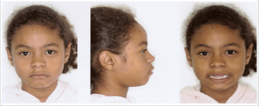
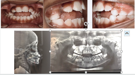
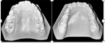
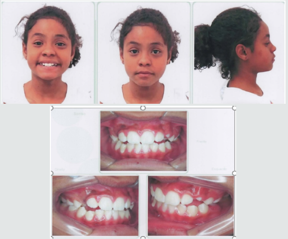
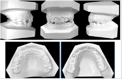
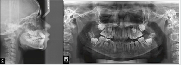
A female patient, 8 years and 4 months of age, melanoderma, came for treatment at the Postgraduate Course in Orthodontics of Brazil University (São Paulo, SP, Brazil). A facial analysis detected convex facial profile, lack of lip closure, and a decrease in nasolabial angle (Figure 1). The patient exhibited thumb sucking habit, mixed breathing, atypical swallowing and speech. shows angle class II malocclusion, 6 millimeters of an anterior open bite, mild crowding and a supernumerary Figures 2&3 tooth in the anterior lower jaw with mandibular midline deviation to the right. Cephalometric Rx shows proclined upper incisors due to the thumb sucking the objetives

Figure 1: Convex facial profile, a decrease in nasolabial angle and the upper lip covering the incisor.

Figure 2: Anterior open bite, mild crowding and a supernumerary tooth in the anterior lower jaw and proclined upper incisors.

Figure 3: Angle class II malocclusion, supernumerary tooth in the anterior lower jaw and an 6mm open bite.

for the first phase of the treatment were to eliminate the thumb sucking, the open bite, dental deviations, provide arch expansion and the extraction of the supernumerary tooth.

Treatment Progress

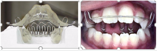
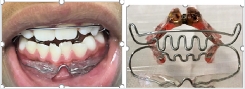
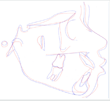
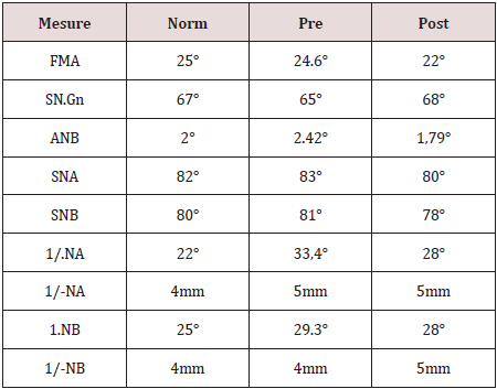
A removable appliance known by Simões Network (SN3) composed with a stainless steel bimaxillary grid (“lower winglets model”) that simulates the incisors occlusion and provides the correct tongue position [15] (Figure 4). The screw was expanded with one-quarter turn biweekly. After 3 months of the treatment beginning o, we added a lip bumper to improve lip seal (Figure 5). We recommended the use for 10 or 12 hours a day. The supernumerary extraction was performed 7 months of the treatment beginning. Figure 6 shows the final of the first stage. Figure 7 shows Angle class I malocclusion and Figure 8 shows the Cephalometric and panoramic Rx after 23 months with the orthopedic appliance. Cephalometric superimposition (Figure 9) and analysis (Table 1) indicated dentoalveolar open bite pretreatment and the correction posttreatment.

Figure 4: SN3 appliance, bimaxillary anchorage with “lower winglets model”.

Figure 5: A lip bumper was added to improve lip seal.

Figure 6: The correction of open bite and the improvement of the alignment.

Figure 7: The arch expansion and molar Class I.

Figure 8: Cephalometric and panoramic Rx after 23 months of treatment.

Figure 9: Cephalometric superimposition revealed maxillary incisor retrusion and mandibular incisor in normal bite.

Table 1: Summary of cephalometric measures.

Discussion and Conclusion

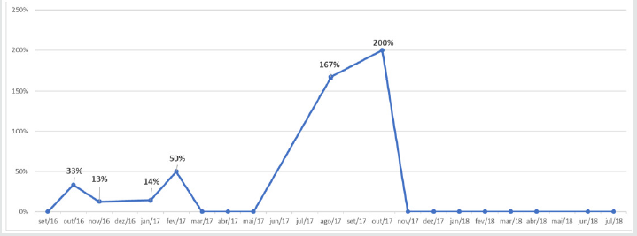
According to the authors, AOB is a challenge daily faced because and it can result speech and swallows’ problems, tongue posture and imbalance between jaw postures [17-19]. Bonna 2016 alerts that the orthodontics or orthopedic devices are fundamental but without family support the habit suppression will not be achieved [20]. The objective for the first phase of treatment were to eliminate thumb sucking, open bite and arch expansion with orthopedic appliance Simões Network SN3 and after a lip bumper was included to improve seal lip. These goals were achieved during the first stage. Graphic 1 shows best fit reduction open bite from May to November 2017. Even pubertal increments offer best time for orthopedic treatment helping determine the predictability, growth direction, patient management and total treatment time, we did not wait to treat because the disadvantages of the open bite [21]. This reported case was successfully treated with SN3 remained stable after the AOB correction. For the second phase with fixed orthodontic treatment will be necessary [22-29].

Graphic 1: Closure open bite variation during time.

Read More Lupine Publishers Pediatric Dentistry Journal Articles:
https://lupine-publishers-pediatric-dentistry.blogspot.com/

Lupine Publishers | Categorical Loudness Scaling in the Fitting of Cochlear Implanted Children

 Lupine Publishers | Journal of Otolaryngology

Abstract

The correct - optimal - fitting of speech processor determines the best result of rehabilitation. The optimal setting of most comfortable level (MCL) is achieved by accurate patient’s assessment of electrical stimuli loudness. Unfortunately, small children can’t give a reliable report about their feelings. How to determine the MCLs in every channel of children implant? Objective methods don’t give the final (optimal) comfort levels of the child’s working program. Therefore, we need subjective assessments. We tried to use a method of categorical loudness scaling (CLS). This article is a guide how to teach CI children to evaluate loudness. Good results of the CLS were observed.

Keywords: Cochlear Implant; Fitting, Categorical Loudness Scaling; C – Levels; Most Comfortable Levels (MCLS); Threshold Discomfort Levels

Introduction

The correct (optimal) fitting of the processor determines the best result of rehabilitation [1]. The optimal settings of C-levels are achieved by accurate subjective patient’s assessments of the electrical stimuli loudness. Unfortunately, young children cannot give a verbal report about their feelings. How to determine the maximum comfortable levels (MCLs) in every channel of an implant in children, i.e. to find threshold discomfort levels? For example, an objective method – reflexometry (registration of stapedial reflex) – is used for fitting of children. But the program in which MCLs are equal to the reflex threshold levels is very rarely optimal one [2].

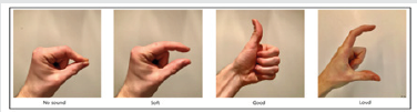
Therefore, subjective estimates of loudness are necessary. There are studies of categorical loudness scaling (CLS) in cochlear implant recipients [3] in which adult subjects participated. Results were reliable ones. What to do with children? We tried to use CLS for assessment of the loudness in cochlear implanted children. The aim of our study is how to find the equal loud C-levels in all channels and using these C-levels to create program with equal loud C-levels. Our study has a practical purpose, so we did not estimate the loudness function. We will not discuss the individual electrical levels of discomfort due to the large differences of these current values between listeners. The CLS is started when we had done reflexometry and parents selected an optimal program. We use our four pictures corresponding to categories “NO SOUND”, “SOFT”, “GOOD” and “LOUD” as a function of the electrical stimulus level (Figure 1).

Figure 1: Four categories of loudness

What reference electrical levels do we use?

Soft Levels

As we wrote earlier, at first day of fitting we approximately defined comfort levels (C-levels) which a child hears as quiet sounds [4].These stimulation levels had been recorded as C-levels in MAP3 of the first configuration. N.B. It is possible that the child did not hear a sound in some channels. Since by the time CLS starts, the child has some experience assessing the loudness of sounds, we can try to clarify these quiet C-levels. We use the first two pictures. This is a part of the CSL already. We stimulate, in our opinion, a quiet signal and “ask”. If child does not hear, we show picture “NO SOUND”. If child hears we show picture “SOFT”. Further, we reduce C-level below the threshold of hearing (2 presses on “Pg down”) and stimulate. We show squeezed fingers – “NO SOUND”. We repeat stimulation on different electrical levels involving the child in this game-study.

Loud Levels

By the time the CLS will be performed at relatively loud С-levels, we had done a reflexometry. How it is performed was described in our article [5]. N.B. In the case of absence of intraoperative ipsilateral reflex, it is impossible to exclude the presence of the contralateral reflex. We created a reflex-program with C-levels equal to the threshold levels of the reflex and recorded it as MAP2 of new configuration. It is known that different children can hear the different intensity of the sounds (from not too loud to loud) at the program where C-levels are equal to reflex threshold levels (our MAP 2). From this reflex-program we had created 3 programs and write them into the configuration. The first MAP is 3 steps lower, and 3-rd and 4-th maps are 3 and 6 steps louder correspondingly. In accordance with our instruction-explanation (“Program is optimal one if your child sometimes hears loud sounds” [6] speech therapists and parents selected optimal (working) program. It should be noted that almost all patients successfully use programs with C-levels above the reflex threshold levels by 3-6 steps (MAP3 and MAP4) [7] and even more. This is normal physiological phenomenon.

When we fit the patient without intraoperative reflex we work in accordance with the standard algorithm of fitting [8]. We gradually increase (in parallel) C-levels at all the electrodes until the parents and we’ll see that some program is loud one. Below this program is a working program (the optimal). Threshold levels are set to 10 percent of C-levels. Using this working program children respond well to all sounds and do not display negative reaction when surrounding sounds are the loud ones. Children can use a louder program in a quiet environment, but a child does not like it in a loud environment (according to parents’ comment). For the purposes of the CLS we use the test program, in which C-levels are less than levels of working program by 3 steps.

Why do we use a program less than optimal one for CLS? The child uses the optimal program in everyday life without problems, but when he will hear a sequence of long-term (300 ms) stimuli with an interval of 300 ms (SWEEP mode) on the one channel at maximal C-levels, the sensation can be unpleasant. N.B. Before CLS, it is necessary to visually assess the child’s reaction to the presentation of single and SWEEP stimuli at the C - levels of the test program - is there any negative reaction? Quite possible that child will not like the maximum C-levels of test program on some channels. C-levels in such channels must be corrected. Corrected C-levels of this test program will be used as loud sounds of the “LOUD” picture.

So. What do we have for our research?

A child hears and orients in sounds in accordance with an information of speech therapists and parents. Parents and teachers have identified a working program that the child uses without problems in all sound environments. Its C-levels are equal (very very rarely) or higher (almost all patients) than threshold levels of stapedial reflex. A child uses CI readily, in the morning the child asks to wear CI himself. A child indicates that the optimal program is the best one. (We asked parents to switch on processor at the first program –the child indicated to change the program). We know approximate loudness of some electrical levels. We know electrical levels, where the child hears quietly. We know where the child hears loudly - at C-levels of the test program. We know where the child hears well- in the area of the third quarter of the dynamic range of the audible current. The child has some experience of distinction between “SOFT” levels and “NO SOUND”. We can start the Categorical Loudness Scaling.

Methodics

How Do We Perform Categorical Loudness Scaling?

We use SWEEP stimulation, i.e. we provide a sequence of identical stimuli of the same amplitude on one channel. The duration of stimuli is 300 ms, the interval between them is 300 ms. SWEEP stimulation is started by pressing down the “Enter” button. The duration of the stimulation is determined by the duration of pressing the “Enter” key and the reaction of the child. We start CLS with a channel with a central frequency in the area of 800-1000Hz. We use categories “NO SOUND”, “SOFT”, “GOOD” and “LOUD” as a function of the electrical stimulus level. At first, we show our fig. 1 to the child. Child already has some experience in categories “NO SOUND” and SOFT”. We show signs with our fingers and explain what the volumes of the sound the child will hear in his (her) head (ear). Owing to our practice, we think that our pictures are more understandable and natural signs for description of child’s own sensation than a circle, squares, cubes etc. These signs are easier to repeat by children. Children may understand meaning of these signs from the birth.

We explain to the child that now we will stimulate, and he will hear a sound in the head (ear). We show the second picture, repeat the sign with our fingers and transmit quiet SWEEP-stimuli. We “ask” the child. If child agrees that he hears a quiet sound, we invite him to show it in the picture or with his fingers. Switching off stimulation, we squeeze fingers, show the first picture, that now there is no signal. Next, we show that we are going to increase the sound. We increase C-levels to 60% of the C-level of test program. We show the “GOOD” picture, raise our thumb and send SWEEP-stimuli. “Ask”. If child agrees, we invite him to show it in the picture or with his fingers. Switching off stimulation, we are clenching fingers, show that now there is no signal. The child agrees. Changing the electrical levels up-down we show with our fingers and on the corresponding picture how loud the signal or no signal will be heard. We invite him to show by his fingers or at appropriate picture. That’s how we perform the CLS training. After some training, a child begins to navigate in their feelings and to give real answers. When we reduce the level of stimulation the child brings own fingers closer, when we increase-move apart. Or they show the corresponding picture. He should be praised. Now we can go to the loudness estimations of the stimuli from the third quarter of the dynamic current range. When a child is assessing of the sound as “GOOD” we “ask” him if it is possible to increase the level of stimulus a little. Waiting for consent or refusal. Many children agree of our offer to slightly increase the stimulation. Then we increase C-level by 1-2 steps, stimulate and look how child displays this increase. Or by fingers, or on pictures. So, we move to the maximal C-levels of our test program where child will hear loudly i.e.to the fourth picture. Closely observe a behavior of the children during the CLS and involve them in the process!

It is curious to note that if some children show estimations of loudness not with their fingers, but with the pictures, they can show their ratings between pictures. For this reason, all four pictures must be placed in one line. Some children begin to show their estimations by the distance between palms. If the child is a contact one and cooperates with the audiologist, you can propose him to increase levels in order to gently touch the threshold discomfort levels. For this purpose, it is necessary to increase a C-levels of test program. But this is the best result. Repeated CLS measurements were done using single-electrode stimuli at a few electrode positions (sometimes all). C-levels at unmeasured electrodes were interpolated. The results were recorded. At the end of the CLS, we set equal-loud C-levels at all channels and make a program. Further, we compare these C-levels with the C-levels of working program defined by parents and teachers. We create new program with C-levels close to C-levels of working program. Since the C-levels of the created program and the working one are not the same ones, we check new program vootiue (on the child’s own ear) and create one program of 3 steps lower and 2 programs by 3 and 6 steps higher. Parents choose an optimal program in accordance with our instruction-explanation [8].

During the CLS we “communicate” with the child, “ask” and “explain”. Naturally, by signs: gestures, fingers, touching, facial expression and praise. We think that such a relationship is interesting to the child - child cooperates with the audiologist, we praise him for his work, correct mistakes, rejoices for the correct answer. Children tend to participate in this “research-game” with interest. We think that children are interested in judging the volume of sounds of different intensity and frequency, that’s why they willingly participate in the CLS.

Discussion

Children work in the CLS successfully. But loudness is a subjective evaluation. Naturally, for example, the same “LOUD” ratings of different patients will be different if they are measured in the terms of SPLs. We believe that the child himself chooses some criteria for assessing the loudness of sound and relies on it for all channels. It is quite natural for each patient to have his criterion, but we hope it is the same one for each child. Somehow it is used in repeated measurements on the different electrodes. Stable repeatable estimates are confirmation of this thesis. Every child adjusted all channels in accordance with own volume criterion. It is clear that adults also have their own criteria too, based on which they assess the loudness of the stimuli. But adult participants themselves noted difficulties in assessing the loudness of singlechannel stimuli of different spectral color. During the development of the fitting program SHCHUP [9] in which the stepped noises are used, adult patients themselves said that the estimation of the loudness of the stepped noises is easier than the loudness estimation of single-channel stimuli. Of course, children have the same difficulties. So, it is clear that the results of CLS on separate channels are not the completion of the fitting of children. The results of the detection equal loud(!) C-levels are important to configure the same equal loud levels in all channels and create a program. Despite the successful mastering of CLS by children, the last step of the fitting is the SHCHUP [9] . SHCHUP is the definition of comfortable SPLs of the stepped noises. The estimation of loudness of the stepped noises is a simpler task for experienced in CLS children too. On the base of SHCHUP’s results, we create four programs in new configuration.

The last step of fitting is the parents’ evaluation of the child’s perception of these programs in different sound environments and the definition of the optimal program in accordance with our instruction-explanation (Petrov & Tsjuk, 2015). Several hundred children (I did not count) participated in procedure of CLS, and I can surely say that the categorical loudness scaling in the fitting of cochlear implant children works successfully. We are sure that CLS is interesting game-procedure for the implanted children and useful method for an audiologist in order to fit children successfully. The CLS is a good encouraging and illustrative program for parents too. For example, we increased the level of stimuli and said mother that sound will be louder now. We stimulate and she sees that her child moves his fingers wider or moves his finger on the fig. 1 to the right. We reduce the level of stimulus and tell mother that sound will be quieter now. We stimulate and she sees that her child brings fingers closer or moves a finger on the fig. 1 to the left. At zero level, child squeezes his fingers together. So CLS is interesting and encouraging procedure for parents - mother sees the coherence of our words about changing of intensity (up or down) and the child response. Mothers are glad that her child correctly assesses the volume of sounds. This article describes General guidelines for performing of CLS. The main aim of this article is to guide how to teach the CI child to assess the loudness of sounds that is very important in the fitting process. Naturally, each child needs his own approach and this CLS, of course, is not done immediately. Speech therapists can use these pictures in their job with implanted patients and hard of hearing children too. Perhaps this method of the CLS can be patented.

Read More Lupine Publishers Otolaryngology Journal Articles:
https://lupine-publishers-otolaryngology.blogspot.com/

Lupine Publishers | Nanotechnology in Phytotherapy: The Effect of Noni’s Nanoemulsion on Bacterial Translocation Induced By Experimental Model of Intestinal Ischemia and Reperfusion

 Lupine Publishers | Journal of Research & Review on Health Care

Abstract

Background: The study evaluated nano structured extract Morinda citrifolia L. (Noni) conveyed in enteral form, in an experimental model of intestinal ischemia/reperfusion (I/R), as well as in the prevention of bacterial translocation.

Purpose: Observe the protective and repairing effect of Noni’s nanoemulsified extract in the presence of induced bacterial translocation, by an experimental model of intestinal ischemia/reperfusion.

Methods and Findings: The study consisted of 2 groups of 7 animals, where the Controls were treated with 0.9% saline solution (I/R + S) and Experimental group (I/R + Noni) treated with 5 mg/ml/Kg Noni nanoemulsion, orally by gavage 12h and 2h before the experiment. In the groups, the superior mesenteric artery was occluded with a vascular micro clamp and the laparotomy reopened 60min. after for pull back the clamp. Treatment response was assessed by blood count, inflammatory markers and biochemical dosages, including a sample of the terminal ileum and hepatic of each animal was harvested, fixed in formalin 10% and included in paraffin and stained with hematoxylin-eosin for morphometric measurement. Measurement of TNF-α, IL-1β, IL-6, and IL-10 was done. One gram of spleen, liver, and mesenteric lymph nodes were harvested for culture by selective means for Gram (-) and Gram (+) bacteria. ANOVA and the post-hoc Turkey and Student´s t test were used, considering p<0, 05 as significant.

Conclusion: Noni´s nanoemulsion positively influenced the organic reactions in the presence of intestinal ischemia/reperfusion, reducing the production of pro inflammatory cytokines, bacterial translocation, preventing tissue injury and attenuating the systemic inflammatory response against the experimental model used

Keywords: Noni: Ischemia-reperfusion injury; Bacterial translocation; Biotechnology; Nanotechnology; phytotherapy

Abbreviations: GGT: Gamma-glutamyl Transferase; ECUA: Ethics Committee on the Use of Animals; NCCAE: National Council for Control of Animal Experimentation; NO: Nitric oxide; AST: glutamic-oxalacetic transaminase; ALT: glutamic-pyruvic transaminase; HSV: total bilirubin and fractions, erythrocyte sedimentation rate; SMA: Superior Mesenteric Artery

Mammography

Intestinal ischemia-reperfusion (I-R) injury is a severe condition resulting from acute mesenteric ischemia, small bowel transplantation, abdominal aortic aneurysm, hemorrhage, trauma, septic shock, or severe burns. Various chemical and cellular mediators have been implicated in the pathogenesis of intestinal ischemia/reperfusion, such as reactive oxygen, cytokines, endotoxins, and neutrophils [1]. Following adhesive interactions among neutrophils and endothelial cells, neutrophil accumulation in the intestinal mucosa contributes to intestinal ischemia/ reperfusion injury via production of reactive oxygen metabolites and proteases. Leukocyte accumulation is a complex phenomenon that also involves endothelium-based adhesion molecules as well as leukocyte chemotaxis factors such as interleukin-8 (IL-8) [2,3]. Intercellular adhesion molecules are normally expressed at a low basal level, but their expression can be enhanced by several inflammatory cytokines such as IL-1β and tumour necrosis factor-α (TNF-α). A variety of cytokines, including TNF-α, interferon-γ, and IL-1β, are released from post-ischemic tissues [4].

It is now considered that these mediators bring about the systemic microcirculatory injury which is thought to be the main mechanism responsible for damage in sepsis. The host defence responses to sepsis may promote the generalized increase in leukocyte recruitment and accumulation in the tissues, which may lead to subsequent endothelial damage, leaky capillaries, and organ dysfunction and failure [5,6]. The organic lesion begins in the lungs, progressing to the anguish respiratory syndrome, followed by kidney and liver failure because of damage caused by the architecture of these organs. Heart failure occurs in late-stage sepsis [7]. The pathophysiology of intestinal ischemia/reperfusion (I/R) in rats with induction of bacterial translocation is widely used in animal models and well established in the literature, and is a viable way of analyzing therapeutic options [8].

The technique will result in a bacterial translocation, generating an ideal model for the therapeutic trial with Noni. Medicinal plants influence the health conditions of the people, in part due to the increase of studies with phytotherapeutics, leading to a confirmation of the therapeutic action of several popular plants, a fact that proves Phytotherapy as part of the culture of the population, being used and widespread for many generations[9-11]. In Brazil, the use of medicinal herbs has its bases in the indigenous practice, which influenced by the African and Portuguese culture, generated a vast popular culture. With the technological advances in allopathic medicine and the pharmaceutical industry in recent years, herbal medicines have been placed in the background, being something allied to popular belief and without scientific bases [12]. However, due to side effects and the high cost of medicines, Phytotherapy is again highlighted and scientific studies with medicinal plants are being resumed [13].

Among the species for herbal treatment highlights the Morinda citrifolia L. (Rubiaceae), popularly known as Noni. Information on its therapeutic benefits has gone through the world causing great demand as a medicinal product [14-16]. Morinda citrifolia L (Noni) has the phytotherapeutic activity of analgesic, antimicrobial, antitumor, anti-inflammatory and antioxidant effects. In scientific studies conducted for the isolation of fixed compounds of the plant, about 200 active substances have already been isolated, where the presence of anthraquinones, triterpenes, iridoids, among others [7- 9]. The anti-inflammatory activity of Noni has been studied in vivo and in vitro by inhibiting the activity of COX-1 enzymes and COX- 2, and the release of chemical mediators from macrophages (nitric oxide (NO) and prostaglandin E2 - PGE-2)[10].

In this sense, products using biotechnology in the form of nanoparticles or nanostructured compounds, can have excellent results, since, due to their reduced diameter, the substance can be used in smaller doses, avoiding the toxic effect of the plant and maintaining its phytotherapic action [11-13]. Thus, the objective of the present study was to evaluate the protective and repairing effect of Noni’s nanoemulsified extract in the presence of induced bacterial translocation, by an experimental model of intestinal ischemia/ reperfusion (I/R) in rats, using the dosage and subsequent blood count, inflammatory markers and biochemical measurements, including histopathological analysis of the compared to the control group treated with 0.9% saline solution.

Material and Methods

Ethical Principles

The experimental protocol was approved by the Ethics Committee on the Use of Animals - ECUA, number 012/2016, Brazil. Animals were handled in accordance with the Guide for the Care and Use of Laboratory Animals, US National Research Council, 1996. The Institutional Committee on Ethics in the Use of Animals approved the research project under the protocol. The care with the use of the animals followed the standards of the Brazilian legislation for the scientific use of animals (Law 11.794 / 2008 National Council for Control of Animal Experimentation - NCCAE / Brazilian Government).

Preparation of vegetable extract hydroalcoholic extract of Morinda citrifolia L: (Noni)

The hydroalcoholic extract of Morinda citrifolia L. was prepared from the aerial parts (stem, leaves, and fruits) of fresh adult plants. The collected material was placed for drying at room temperature; then comminuted with a knife and placed for 24h in an oven at a temperature between 45ºC and 50ºC to remove moisture. It was then subjected to a grinding process to obtain the powder. This material was weighed and deposited in a glass vessel with the addition of 70% hydroalcoholic solution in the ratio of 1:3 of the powder. The resulting mixture was stirred for 12h and stirred for five minutes every two hours under two simple filtration procedures under reduced pressure to give the crude extract, which was concentrated in a rotary evaporator under reduced pressure, at a temperature between 55°C and 60°C, for total solvent elimination. The product obtained after concentration was in the form of a paste which was diluted in distilled water until a hydroalcoholic extract at the concentration of 5mg/ml was obtained, being kept in a refrigerator at 10ºC until it was used.

Obtaining Nanoemulsified Systems

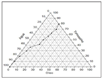
Nanoemulsion systems were obtained by maceration in a mixture of ethanol: water (8:2/800mL of alcohol 70° INPM + 200mL of distilled water) according to the previously described methodology. The study of phase diagrams of the oil, water and surfactant mixture formed a nanoemulsified (SN) system with a self-emulsifying characteristic. The SN system was considered O/W of the autoemulsifying type due to the unchanging of its appearance after successive dilutions in water. The vegetable oil used contains the following chemical components: vitamin E, oleic, linoleic and linolenic acid, low saturated fat and high content of polyunsaturated components [17,18]. The procedure used to obtain the nano emulsion regions is based on the method involving the determination of the maximum solubility points of active matter (surfactant) in the aqueous and oily phases, by means of mass titrations. The structure is composed of vegetable oil in the range of 0.5% to 6.0%; a surfactant in the range of 8.0% to 20% and distilled water in the range of 75% to 90% (Figure 1).

Figure 1: Phase Diagram (Maciel 2009).

Description of Nanoemulsion Preparation: Initially, industrialized vegetable oil was weighed on a precision digital scale (model: FA-2104N / 2008; Brand: BIOPRECISA-->) in the preferred range (1% to 5%), the surfactant in the preferred range (8% to 20%), and distilled water in the preferred range (75% to 90%) mixed and heated the components of the formulated SME - Nanoemulsion System, in magnetic stirrer with heating - stirring range 100-2200rpm and temperature controlled in the preferred range between 40°C to 70°C (Model NI1103P/2009: Mark: NOVAINSTRUMENTS-->). Thereafter, centrifuged at a constant speed, between 550rpm and 650rpm, for a preferential time of 15 minutes. (Model TDL80-2B, Mark Centribio-->).

Analysis Characterization: Performed through the refractive index, droplet diameter, rheological behavior and surface tension. To obtain the refractive index, an analog bench refractometer (ABBE, Model: 2waj; Mark: BioBrix-->) was used at a temperature in the range of 20°C-30°C.

Determination of droplet diameter: The diameter of the nanoemulsion droplets was determined by measurements in triplicates and with the refractive index of 1.4715 with a light beam of 659nm wavelength and angle of incidence of 90°. The diameter of the droplets (ranged from 50nm-75nm).

Rheology: The evaluation made from the graph generated by shear stress versus shear rate using a greenhouse thermometer (HG - Brazil, No.1876/11-->), in the range of 20°C-30°C, with variation for the shear rate (1s-1-1000s-1), resulted in a linear behaviour, with r2 = 0.91058.

Fluid Classification: The fluid under analysis was classified as Newtonian and the viscosity was determined to be 2mPa.s - 6mPa.s (2cP - 5cP).

Maximum Dilution Analysis: The evaluation was performed by experimental data of surface tension. Assays were performed using the SensaDyne Tensiometer apparatus (model QC-600, Chem-Dyne Research Corp. - USA). The description of the method consisted of measuring the maximum bubble pressure using two capillaries with holes of different diameters, where an inert gas (N2) was pumped at a certain constant pressure (200-595kPa). The larger capillary measured the effect of the immersion depth and the smaller the surface tension. For each measurement, the samples were diluted in distilled water, with concentrations varying until the values of surface tension close to the water (γH2O = 72.1mN/m) and temperature in the range of 20°C to 30°C were reached.

Surgical model / experimental design: We used 14 Wistar male Wistar rats weighing 265±32g (from Nucleus of Experimental Surgery, Potigura Universty - LAUREATE INTERNATIONAL UNIVERSITIES - UnP/Natal/Rio Grande do Norte State/ Brazil), randomly divided into 2 groups, kept in individual cages with food and water standard (Labina-Purina-->) is rodents, ad libitum. In the experimental group (n=7) rats received 5mg/mL/Kg (EMS-FC5) Noni nanoemulsion via the probe/gavage 18 and 2 hours prior to clamping of the superior mesenteric artery (I/R), the remainder rats (n=7) were treated with oral saline solution at 0.9%, 18 and 2h prior to (I/R). After 12h of fasting, the rats were anesthetized with for the induction of anesthesia general, the solution of Zoletil--> 50, the anesthetic dissociative, will be used in the dose of 0.3mL/100mg intramuscularly in the region of the quadriceps, with disposable syringes of 1mL of insulin and needle 27F and operated under aseptic conditions. In groups I/R + Saline and I/R + Noni, under sterile conditions.

Measurement of bacterial translocation: After shaving, the abdominal skin was disinfected with 0.2% chlorhexidine. All procedures were performed under sterile conditions. A laparotomy was performed and the superior mesenteric artery (SMA) was occluded with a microvascular clamp for 60 minutes. In order to block any collateral blood supply, the right colic and proximal jejunal arteries were also clamped. The laparotomy incision was then closed, to be opened later for removal of the clamps after 60 minutes of ischemia. Reperfusion was confirmed by the return of the mesenteric arcade pulsation. The incision was closed again and the animals were killed by anesthetic overdose (thiopental 100mg/ Kg) after 120 minutes of reperfusion. They breathed spontaneously throughout the procedures.

Measurement of bacterial translocation: At the end of the procedures (time = 180 minutes), a midline laparotomy was performed under aseptic conditions and biopsies were aseptically obtained for bacterial colony counts. One gram of mesenteric lymph node complex, blood, liver, and lung were removed for culture. Tissues were homogenized and aseptically solubilized after addition of 0.5mL of 0.9% saline. Aliquots of 0.2mL were processed and cultured on selective MacConkey’s agar and Blood Agar for detection of gram-negative and gram-positive bacteria, respectively. The agar plates were incubated at 37oC and examined for growth after 24 and 48h. Any growth in the plates of bacteria of the same biotype as cultured was considered positive and expressed as colony-forming units per gram of tissue (CFU/g).

Laboratory analysis/ Cytokine Assays: After 24h of a conclusion of the procedures under anesthesia and aseptic conditions, blood was collected by cardiac puncture to measure the hemogram, hepatogram, cytokines, and albumin. Samples of blood were treated with EDTA and the plasma was separated by centrifugation at 2000rpm and stored in -80°C for later measurement of tumor necrosis factor (TNF-a) interleukin-6 (IL-6) and interleukin- 1b (IL-1b) by the ELISA (enzyme-linked all immunoassay kits from PeproTech--> (Rocky Hill, NJ, USA) according to the manufacturer’s recommended protocols. The fluorescence was measured by a Bio-Tec--> Instruments EL808 ultra microplate reader, using KC4-V3.0 analysis software. The sensitivity of detection was 30pg/mL for all cytokines. For counting leukocytes and red cells using an automated cell counter (Abbott Cell-Dyn 3500R CD--> 5L-3500, USA). For albumin, alkaline phosphatase, gamma-glutamyl transferase (GGT), glutamic-oxalacetic transaminase (AST), glutamic-pyruvic transaminase (ALT), total bilirubin and fractions, erythrocyte sedimentation rate (HSV) blood was treated with EDTA.

Histological study: Terminal ileum and liver specimens were fixed in 10% buffered formalin and embedded in paraffin. Sections cut at a thickness of 4μm were stained with hematoxylin and eosin for morphometric measurements using an image analyzer (Image- Pro Plus, Media Cyber-->)[19-21]. The damage of the intestinal specimens was assessed in a blinded manner by an experienced pathologist according to microscopic criteria for degree of damage based on a grading system previously described: normal mucosa, 0; subepithelial space at the villus tip, 1; more extended subepithelial space, 2; epithelial lifting along villus, 3; denuded villi, 4; loss of villus tissue, 5; crypt layer infarction, 6; transmucosal infarction, 7; transmural infarction, 8.

Statistics: Data analysis was performed using the BioEstat--> 2.0 program. Differences between the microbiological samples as measured by positive cultures were evaluated by a test for differences between proportions. The results were tabulated and compared by ANOVA using post hoc analysis with Tukey and Student’s t test. P<0.05 was considered significant. Data on continuous quantitative variables are the mean ± expresso standard deviation. In the variables that did not present normal distribution, the logarithmtransformation method was adopted. These variables are represented by their respective logarithms. To verify if the differences between the Experimental (Noni nanoemulsion) and Control groups were statistically significant, the Student’s t-test for independent samples was used. The statistical package SPSS-->21 was used.

Results

We observed bacterial translocation to mesenteric lymph nodes, liver, lung, and blood in all animals subjected to I / R. However, in I/R group rats treated with Noni nanoemulsion, translocation to these organs and blood was significantly lower than in I/R untreated (Table 1). Cytokines had lower levels of proinflammatory cytokines in group I/R+Noni (TNF-α, IL-1β, IL-6) and a higher level of antiinflammatory-cytokine (IL-10), when compared with I/R + Saline (C) (Table 2). In I/R + Saline (Control) group rats, the levels of pro-inflammatory cytokines were significantly higher when compared to I/R+Noni. This group had the highest values of IL-10 when compared with (Control) group (p<0.05). Noni was able to maintain and modulate the inflammatory reaction in the experimental group, which was proven through normality in the hematological dosages. There was also a significant reduction in the number of total leukocytes, which did not generate immune suppression in experimental animals, but control the systemic inflammatory response in the presence of induced bacterial translocation for intestinal ischemia and reperfusion.

Table 1: Bacterial Translocation in groups treated and not treated with Noni nanoemulsion (colony-forming units per gram of tissue - CFU/g).

*p < 0.01 compared with groups I/R + Saline (C) and I/R + Noni nanoemulsion.

Table 2: Serum levels of cytokines in groups with and without Noni nanoemulsion treatment.

*p< 0.01 compared with groups I/R + Saline (C) and I/R + Noni nanoemulsion.

Table 3: Descriptive and inferential statistics of hemograma results.

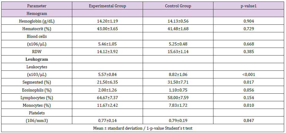
Figure 2: The mucosa is injured, and leukocyte infiltration of lamina propria and mucosa are shown (group I/R), 100x. 2: Hemorrhage and inflammation of mucosa (group I/R), 100x.

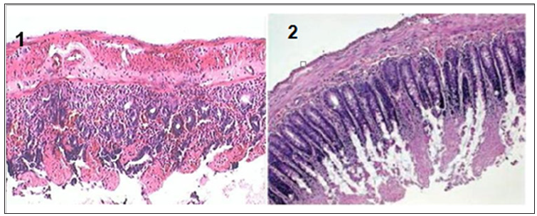
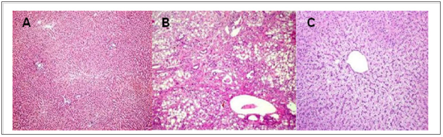
A trend towards normality was observed in the other cellular parameters measured in relation to the control group (Table 3). Macroscopically, the segments of the organs studied presented intramural dilation and hemorrhage, with greater intensity in rats of the I / R group, compared to the experimental group (Noni). Microscopic findings revealed marked mucosal lesion after ischemia and reperfusion injury; we observed more intense lesions in the rats of the I / R group compared to the other groups. The most frequent lesions were: disorganization of the normal tissue structure, transmural infarction, infiltration of leukocytes in the lamina propria and mucosa, alveoli and hepatic sinusoids. In the group that used the nanoemulsion of Noni, there was protection and preservation of the tissue structure, with reduced or absent infiltrating inflammatory reaction (Figures 2-4).

Figure 3: Preserved intestinal mucosa, demonstrating normal villi and intestinal epitelial cells of uniform pattern, normal to histological examination, 100x

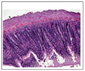
Figure 4: A) Normal liver structures are demonstrated. B) A hepatic section from a septic rat with vehicle (normal saline) treatment. Patches of hepatocytes show necrosis with eosinophilic cytoplasm nuclei that are condensed and intensely stained with hematoxylin. C: A section from a septic rat with Morinda citrifolia L (Noni) treatment. Liver structures appear normal. (HE.50;100 x /100 μm).

Discussion

The present study used an experimental model of ischemia and reperfusion, to verify the effect of nanostructured extract Morinda citrifolia L. (Noni) on intestinal injury and bacterial translocation. Some authors consider the bacterial factor, crucial in the pathogenesis of sepsis and multiple organ failures [22]. In surgery and intensive care, intestinal obstruction and intestinal ischemia are the most associated pathological conditions [23]. The use of medicinal plants for the treatment of diseases has been occurring since the dawn of civilization. The development of methodologies for the isolation of active substances has made it possible to identify substances in complex samples such as plant extracts. In this way, the interest for compounds of vegetal origin that could be used as prototypes for the development of new drugs resurfaced [24]. Medicinal plants represent the main raw material used for the synthesis of medicinal products, besides being used as therapeutic agents. Plant consumption is overvalued in traditional use based on it medicinal benefits [25].

Noni (Morinda citrifolia L.) has become a promise of the cure for a variety of diseases, ranging from simple hypertension to malignant tumors; even provokes the cure of syndromes, still incurable such as AIDS and other viral diseases [26]. However, The popular use and wellbeing attributed to Noni make the industry commercially explore Morinda citrifolia L products, often without scientific evidence [15].In this context, the use of biotechnology transforming Noni into a nanostructured compound, has the advantage of using the plant’s medicinal properties, reducing its toxicity, keeping its bioactive principles beneficial to health [27,28]. Antimicrobial activity of Noni has already been reported in the literature. Studies have shown that noni inhibited growth in vivo and in-vitro bacterial strains such as Staphylococcus aureus, Pseudomonas aeruginous, Bacillus subtilis, Escherichia coli, Helicobacter pylori, Salmonella and Shigella.

In addition, Noni has already been studied on its effect against Plasmodium falciparum, believed to be due to the presence of anthraquinones, acubin, L-asperuloside, alizarin, scopoletin, among other substances [29,30]. It has also been found that ethanol and hexane extracts of noni have an antitubercular effect since they inhibit by 89-95% the growth of Mycobacterium tuberculosis. The major components identified in the hexane extract were E-phytol, cycloartenol, stigmasterol, b-sitosterol, campesta-5,7,22-trien-3-bol, and the ketosteroids, stigmasta-4-en-3-one and stigmasta-4-22- dien-3-one[18-20]. Moreover, they showed that the anti-microbial effect is highly dependent on the stage of ripeness and on processing, being greater when the fruit is ripe, without drying [23-25]. The limiting factor for the use of Noni as an herbal remedy is that most of the studies previously found in the literature, administer the extract in the alcoholic or hydro-alcoholic form, which may, through prolonged use, mainly cause hepatotoxicity [24].

With this in mind, the present study makes its scientific contribution to demonstrate that with the use of biotechnology in the formulation of a nanostructured extract of Noni, such undesirable side effects were abolished, maintaining the active principles of the vegetable under analysis [31]. Recent studies have demonstrated, respectively, the efficiency of Noni´s nanoemulsion in experimental models of healing of infected wounds in the skin of rats as well as in abdominal sepsis induced by cecum ligation and puncture [32,33]. This phenomenon was confirmed in the present study, where a reduction in the total leukocytes and polymorphonuclear levels was observed, maintaining normal hemoglobin and hematocrit levels in the experimental group, which used Noni in the presence of an experimental model of intestinal ischemia/reperfusion (I/R) in rats with induction of bacterial translocation.

Conclusion

In conclusion, the present study demonstrated that Noni’s nanoemulsified extract acted as an immune modulatory agent in the presence of an experimental model of intestinal ischemia/ reperfusion (I/R) in rats with induction of bacterial translocation, reducing the systemic inflammatory response, stimulating the immunity of experimental group animals, preserving liver function and maintaining its bioactive principles beneficial to the experimental model used.

Read More Lupine Publishers Research & Reviews Journal Please click on below link
https://lupinepublishers.blogspot.com/ 

Lupine Publishers | Scientific Student Societies: A Way of Scientific Research Vocations Boosting

 Lupine Publishers | Journal of Surgery & Case Studies

Abstract

Born in Russia at the end of the XIXth century the Scientific Student Societies have developed a rather original way of initiation and involvement of the young in the scientific research during High School and University cursus. All through the XXth century and up to now, they have given several generations of Russian scientists an adequate pre formation consisting not only of skill acquisition in their future speciality but also in planning, realization and organization of scientific research and sharing of its results. Their popularity was also due to the high degree of initiative and autonomy left to the students.

Abbreviations: SSS: Scientific Student Societies

Introduction

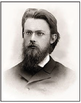
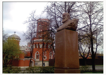
In our days, when most of young people with a diploma of physician are no more inspired by a scientific career possibility, and though Occidental World has general negative opinion about Russia and its institutions, it is not forbidden to exhume some moments which have proved efficacy and may be useful for.com now. Such an interesting institution (from my point of view) was the Scientific Student Societies (SSS) [1], existing in all the High Schools and Universities, but may be especially activated in Medicine Faculties. They were created in the end of XIXth century by famous scientists such as VI Vernadski (Figure1) and his colleagues in Sankt Petersburg (1882) and in the beginning of the XXth century by NE Jukovski (Figure 2) in Moscow (1909) [1-4]. In the 30-ies they were reactivated and widespread through all the country. After the 2nd World War, SSS were also working in the other countries of the “East Bloc”. The links and experience exchanges were current between them (International meetings and conferences, scientific information share, student exchanges and so on). Presently in the XXIth century they have not disappeared: “NIRS” - student scientific research work - remains a preoccupation of the academic staff in Universities and High Schools as well as different Ministries of the Russian Federation. Student scientific associations still exist, may be a little modified, sometimes independently as “Meridian”, “Luch” (that means ray or beam). Books including scientific articles written by students are still published [5-7], regional and national competitions are organized.

Figure 1: Vladimir Vernadski (1863-1945) famous chemist and mineralogist, creator of the first student scientific circles in Russia.

Figure 2: Monument to NE Jukovski (1847-1921) - The “Father of Russian Aviation” - in the Entry Square of the Petrovski Palace (Aviation school) in Moscow.

Description and Commentaries

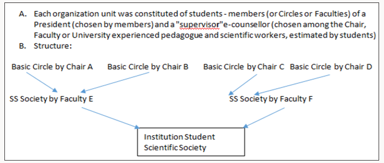
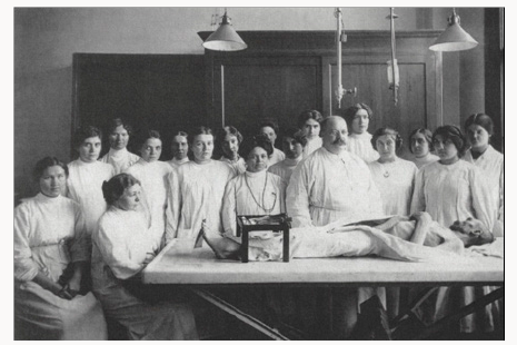
The SSS aims were: to popularize scientific research among students, to find out the most talented among them and to help them to develop towards an eventual scientific career. It was also a mean for students to acquire deeper knowledge in one or several disciplines and to choose their future speciality. The Student Scientific Circles eventually provided the departments with qualified helpers, as a just return for the teaching staff mobilisation during the young researcher’s formation. The structure schema of the SSS is presented in Figure 3. At the basis level was the Circle. As soon as they wanted, students were invited to join a student scientific circle by the department of their choice and to begin their initiation according to their trends with one of the assistant or docent. At this level, the students learned step by step how to manage scientific literature, to review it, to deepen their knowledge’s in the chosen subject, to acquire technical skills and, last but not least, to participate to the research of their mentor/supervisor, or even to start their own investigations on their personal research topic.*NB. The work performed within the SSS activity differed from end of cycle obligatory works, but the members of SSS were allowed to include their personal data in the end of cycle work, if it was adequate. The students - members of a circle - elected their president - responsible who organized periodic reunions for reviewing the work performed by the circle members. During these meetings experienced assistants and docents or professors were invited to present lectures or demonstrations helping the students to assess the peculiarities and the research specifics of the discipline (Figure 4). The best student ‘works were selected and recommended for reporting at Faculty and inter Faculties student scientific conferences.

Figure 3: Schema of a Student Scientific Society structure.

Figure 4: Professor SHOR GV (1812-1944) - well known Pathologist - with students at a meeting of the student scientific circle of Pathologic Anatomy in the 30-ties.

The next level was Faculty and University or High School Scientific Student Society. The department circles joined forming faculty and institute Student Scientific Societies (SSS), which were gathered as University or High School SSS. They were handed by students and only supervised by a responsible chosen among docents and professors of the Faculty. Students elected their president and delegates for contacts with other faculties, institutes of the country and of foreign countries. They organized faculty conferences, Inter-faculty scientific sessions. Their activity was financed either by the Professional Union of their School or by the University budget. The most promising students - members of SSS were further recommended for scientific work either in the department where they started their work, or in Scientific Research Institutes and other High School Faculties (according to the young specialist’s will and the possibilities of the aforementioned institutions). The Ministries took into account the SSS activity of the young specialist when his future was considered after the end of his cursus. Besides career start consideration, other awards were current: scientific books, scientific travels, being the co-author of a “chief’s paper, and so on. So the students made acquaintance not only with the individual searching process itself (Figure 5), but also with elements of organizing scientific research, co-operative investigation, discussion and peer evaluation of its results both by other students and by the Faculty staff scientists. Students also learned to communicate at different levels and, if they wanted, to prepare themselves to a scientific career. If not, nevertheless the aptitudes obtained during their work in the SSS was precious for their further professional activity: acquaintance with special literature research methods, reviewing and critics of scientific publications, acquisition of some technical skills, capacity to plan scientific research and organize scientific meetings.

Figure 5: Students at Research work in a Technical High School in the 80-ies.

It is estimated that about 20% of the students attended the SSS. Among them about 30% have presented a valuable work (compilation, fundamental or applied research). Most of the exmembers of SSS have pursued a career in the previously chosen specialty. In Russia, all through the years 1930-1990 and up to now most of those who have followed a successful scientific or pedagogic career, were ancient members of the SSS. (That does not mean that without SSS a scientific career was not possible). Many of the students, even foreigner hosts, who have passed through this “school” have been later eminent scientists of their countries (for instance: Academician VI Shumakov - the first Director of the Transplantation Institute in Moscow, Professor VM Filipov - present Rector of the Russian University od People Friendship; Professor R Roman Ramos - Dean of the Medicine Faculty of the Mexico Autonomous University)

Conclusion

The SSS have given several generations of motivated Russian scientists an adequate pre formation consisting not only of skill acquisition in their future speciality (especially precious in surgical disciplines) but also in planning, realization and organization of scientific research and share of its results. This was capital for a developing country and remains important nowadays. The large autonomy and initiative given to the students in the SSS has certainly contributed to their popularity and success. This experience ought to be adapted to the conditions of our present society development and could enhance individual initiative and motivation, as well as collective research organization. It ought to be included into Faculties staff task and financing.

Read More Lupine Publishers Surgery Journal Article:
https://surgery-casestudies-lupine-publishers.blogspot.com/

Lupine Publishers | “Role of Agriculture in Ayurvedic Drug Research”

  Lupine Publishers | Current Investigations in Agriculture and Current Research

Mini Review

Ayurveda which is known as science of life, is beauty of Indian culture. From ancient era Indian people live this science. Ayurveda given first preference to prevention than cure. Bhaishajya (doctor), Rugna (patient), Aushadha (medicine/drug), Parichrka (medical assistance) is four chikitsapaad of chikitsa [1]. Aushadha (medicine/ drug) is one of the important chikitsapaad among them. Nowadays golden days of Ayurved are arrives. CCRAS and AYUSH all are engaged in Ayurved research. There are four types of research, drug research is one of important research among them. Drug research in Ayurved done with modern as well as ancient parameter. For drug research source of plants is necessary. Original raw material of herbal drug can supply from special Ayurvedic agriculture. Drug research include proper identification, lit. study, filed work, cultivation, collection, testing efficacy of various part and body of plants, adverse effect, adulteration, morphology, photochemistry, study of various formulation and testing action of drug. [2].

In farming India has second rank in whole world. Due to various climate, soil, geographic structure variety of vegetable, fruits, plants production occurs in india.in exporting also our country is at top rank [3] India has shown a steady average nationwide annual increase in kilograms produced per hector for some items of agriculture. For treatment Ayurvedic physician need different types of fresh and qualitative drugs. Unfortunately most of drugs are unavailable or available with adulteration. Due to popularity of Ayurveda demand of herbal drugs is increased, but supply are less as per need, so marketing peoples do adulteration in herbal drugs. If raw so material of medicine is not pure, than how can we expect proper results? So, there is need of development of trained agriculture filed as per medical Science i.e Ayurveda.

Read More Lupine Publishers Agriculture Journal Article:

https://lupinepublishers-agriculturalsciences.blogspot.com/

Lupine Publishers | Economic Analysis of Poverty Status of Small-Scale Farmers in Bayelsa State, Nigeria

    Lupine Publishers | Current Investigations in Agriculture and Current Research

Abstract

The study analyzed the household poverty status of small scale farmers in Bayelsa State, Nigeria using a multi-stage random sampling technique to sample six hundred farmers. Data were collected using structured questionnaire and were analyzed using descriptive statistics, FGT [1] index and the logistic regression model. The result revealed that the majority of the farmers 80% were females, while 79% of the respondent was married with 46% of them having no formal education. Twenty-seven (27) percent of the crop farmers are poor while thirtyeight (38) of the livestock farmers were poor. Also, the poverty depth and severity of crop farmers were 0.072 and 0.038 respectively whereas they were 0.098 and 0.052 respectively for the livestock farmers. The logistic regression model revealed that age, educational level, household size, farming experience, farm/herd size, household income, household expenditure and membership of cooperative contributed significantly in determining the poverty status of the farmers. This study therefore recommends measures needed to be put in place to encourage and improve the welfare of the farming household towards productive and sustainable agricultural development for poverty reduction.

Keywords: Economic; Poverty; Status; Small Scale; Farmers

Introduction

Nigeria is a vast country endowed with substantial natural resources which include; 68 million hectares of arable land, fresh water resources covering about 12 million hectares, 960 million hectares of coastline and ecological diversity that favor the production of a wide variety of crops, livestock, forestry and fisheries product [2]. These coupled with its 37 million hectares of natural forest and rangeland and total land mass of 923,768km2 [3] makes agriculture one of the prominent sub-sector. In spite of these resources’ endowment, the productivity of agriculture continues to dwindle. One of the major problems confronting Nigeria today is how to improve the quality of life in the rural areas and reduce the level of poverty [4]. Poverty in Nigeria is not only a state of existence but also a process with many dimensions and complexities [5]. The report of the 2006 Nigerian Core Welfare Indicator (CWI) on the poverty profile in the country stated that the dependency ratio, which was defined as the total number of household members aged 0 – 14 years and 65 years and above to the number of household members aged 15 – 64 years was 0.8 Central Bank of Nigeria [6]. This indicated that almost a one-to-one dependency ratio and reflected the high population growth rate in the country. There is also large income inequality with the top 10% of the income bracket accounting for close to 60% of the total consumption of goods and services [7].

The World Bank [8] describes poverty to comprise of many dimensions. It includes low incomes and the inability to acquire the basic goods and services necessary for survival with dignity. It encompasses low levels of health and education, poor access to clean water and sanitation, inadequate physical security, lack of voice and insufficient capacity and opportunity to better one’s life. It may also result in not having enough capacity to feed and clothe the family and/or earn a living. About 90% of the country’s food is produced by small scale farmers cultivating tiny plots of land who depend on rain fed agriculture [9]. According to Omonona [10], poverty is pervasive although the country is rich in human and material resources that should translate into better living standard. Despite its plentiful resources and oil wealth, poverty is widespread in Nigeria [11]. The situation is said to have worsened since the late 1960s, to the extent that the country is now considered one of the 20 poorest countries in the world. Over 70% of the population is classified as poor, with 35% living in absolute poverty. Poverty is especially severe in the rural areas, where social services and infrastructure are limited or non-existent. Majority of those who live in rural areas are poor and depend on the agriculture for food and income.

The concern on the threat posed by poverty has led the Nigerian government over the years to devote considerable attention to alleviating its scourge through various policy projects and programmes which seems not to have stem the ugly situation till date. In view of these, the question about the poverty status of rural dwellers especially the small scale farmers remained unanswered. It is on this premise that this study was carried out to answer these questions.

a) What are the socio-economic characteristics of these small scale farmers?

b) Are the small-scale farmers really poor?

c) What are the factors influencing poverty status of the small scale farmers? and

d) What options are available to small scale farmers in reducing their poverty levels?

Thus, the main objective of this study is to evaluate the poverty status of small scale farmers in Bayelsa State, Nigeria. The specific objectives are to:

a) Describe the socio-economic characteristics of small scale farmers.

b) Compare the poverty status of crop and livestock farmers in the study area;

c) Determine the factors influencing poverty status of the farmers; and

d) Make policy suggestion towards poverty alleviation.

Methodology

Study Area

The study was conducted in Bayelsa State, Nigeria. It is located between latitude 5° 00¹ to 10° 30¹ N and longitude 4° 55¹ to 6° 00¹ E and covers an estimated land area of 1,810km² with a population of about 856,729 thousand [12]. It shares local boundary with Delta State, Anambra State and Rivers State with the Bight of Benin at the Southern Flank. There are eight (8) Local Government Areas (LGAs) in the state with Ijaw as their major language. Mean annual rainfall of the area is 2,200mm for upland or dry regions where water bodies are few and 3,500mm for wetland or lowland region which comprises of land areas being surrounded by water bodies. Temperature range is between 23 – 31°C and vegetations found in the area include the saline water swamp, mangrove swamp and the rain forest. Major seasons are the dry (November – February) and wet seasons (October – March). Also, the seasonal condition of the area presents a healthy environment for farming which is the main source of income and livelihood of the state’s population and agriculture accounts for about 72% of the labor force.

Sampling Procedure and Sample Size

The sampling involved a multistage random sampling technique. Firstly, six (6) local government areas were randomly selected using the proportionate sampling method at 75% precision level from the purposively selected three (3) agricultural zones according to Agricultural Development Programme (ADP) structure. In the second stage, ten (10) villages were also randomly selected from the six (6) LGAs each making a total of sixty (60) villages. The third stage involved a simple random selection of five (5) crop and five (5) livestock farmers each from the villages using the list provided by ADP from each of the villages. A total of six hundred (600) respondent farmers were used.

Data Collection

Both primary and secondary data were used for the study. The collection of primary data was achieved using a set of structure questionnaire that was administered by the researcher and trained enumerators complemented with oral interview, information that was collected covered the areas of socio–economic characteristics, farming operations, and income and expenditure patterns. Secondary data were sourced from relevant material both published and unpublished.

Analytical Technique

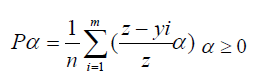
Three analytical tools namely; descriptive statistics; Foster, Greer and Thorbecke (FGT) model of poverty decomposition [1]; Logistic regression were used for the study. Descriptive statistics such as frequency, percentages, mean were used to profile the socio-economic characteristics of the farming households and also to present the results of the findings. The FGT measure was used to assess the incidence, depth and severity of poverty of the farming households. The approach makes use of the aggregate values of the poverty indices – poverty headcount, poverty gap, and squared poverty gap. The use of the FGT measures required the definition of poverty line and this was calculated on the basis of aggregated data on household income. The FGT measure as used by Baiyegunhi and Fraser [13] is expressed as:

Where:

z = Poverty line

m = Number of households below poverty line

n = number of households in the reference population

yi = Per adult equivalent income of ith household

α = Poverty aversion parameter

z-yi = Poverty gap of the ith household

z – yi = Poverty gap ratio

The headcount index was obtained by setting a = 0, the yield poverty gap index when a = 1, and squared poverty gap index when a = 2. The poverty line is a predetermined and well defined standard of income and value of consumption. In this study, the poverty line was based on the income of the households. A relative poverty line was used in which a household was defined as poor relative to others since they are all farmers. Two third of the mean per capita income (MPCI) was used as a moderate poverty line while one third was taken as the line for extreme poverty. Thus, the farming households were grouped into three categories based on their levels of poverty: the extremely poor (those whose income was less than one-third of MPCI), the moderately poor (those whose income lies between onethird and two-third of the poverty line) and the non-poor (those whose income was above two-third of the poverty line).

Adult equivalents were generated following Nathan and Lawrence [14], thus:

AE =1+ 0.7(N₁ −1) + 0.5N₂

Where

AE = Adult equipment

N₁ = Number of adults aged 15 years and above

N₂ = Number of children aged less than 15 years.

Logit Regression Model

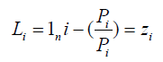
A binary logistic regression model was used to analyze the determinants of poverty. Thus, poverty is the dependent variable and is determined by independent variables such as socioeconomic characteristics of households and access to services. The dependent variable is binary (1 if the household is poor and 0 if the household is non-poor). The logit model is based on the cumulative logistic distribution function expressed as:

Where:

L_i = log of the odd ratio, which is not only linear in Xi but also linear in the parameters,

P_i = is the probability of being poor and ranges from 0 to 1.

Z_i = the function of the explanatory variables (x) which is expressed explicitly as:

Where:

Bo = Intercept, Bi – B₉ = coefficient of the independent variables, xi = is the vector of relevant independent variables and U = is the stochastic error term, z = the dependent variable defined as the mean annual per capita expenditure. It was measured in binary terms such that 0 = poor, that is if the mean per capita household expenditure is below the poverty line and l = not poor, that is if the mean per capita household expenditure is above the poverty line and:

X₁ = Age (number)

X₂ = Farm size (number of herds/hectares)

X₃ = Marital Status (1 = Married, 0 = otherwise)

X₄ = Household size (number)

X₅ = Education Level (number of years)

X₆ = Major Occupation (1 = farming, 0 = otherwise)

X₇ = Farming Experience (years)

X₈ = Household income (Naira)

X₉ = Household Expenditure (Naira)

X₁₀ = Extension contact (1 = yes, 0 = otherwise)

X₁₁ = Cooperative Membership (1 = yes, 0 = otherwise)

Results and Discussion

Socio-Economic Characteristics of Respondents

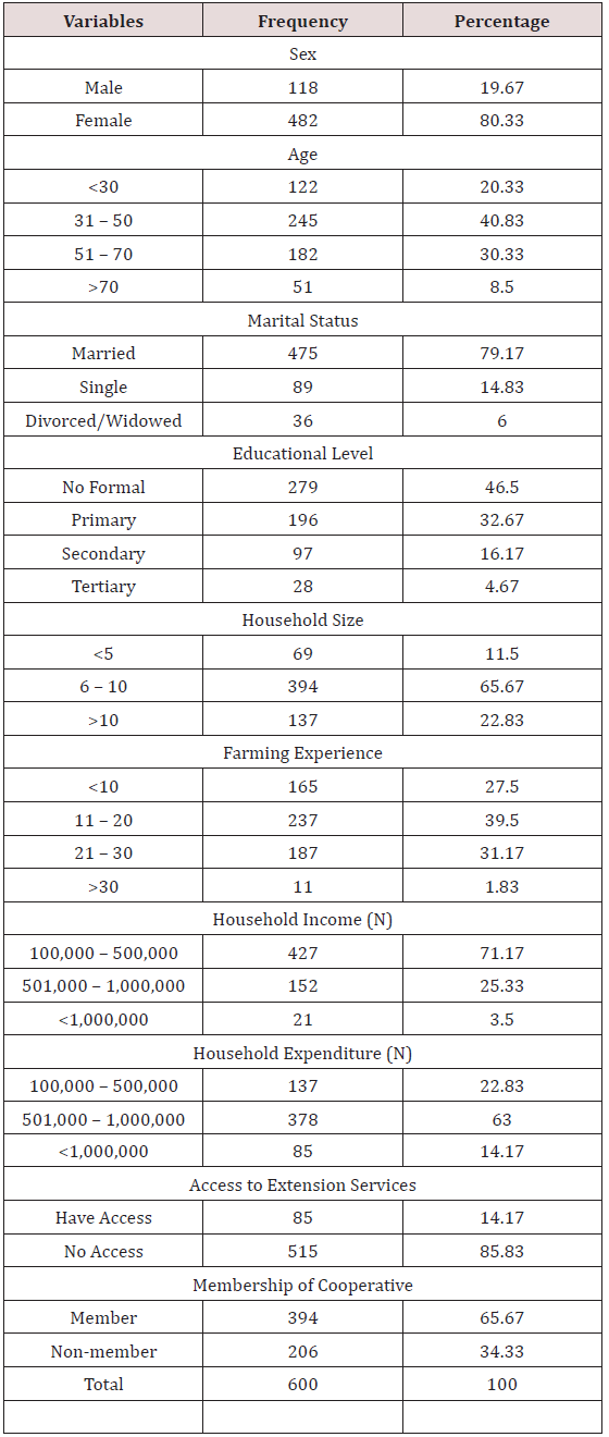
Table 1 shows the socio-economic characteristics of the respondents. The majority, 80.3% of the respondents were female while 19.7% were male. This suggest that majority of small scale farmers in the study area are female. About 61% of the respondent were age <30 to 50years with the mean age of 41 years. These results suggest that majority of the farmers were in their active productive age. Moreover, 79.17% of the respondent farmers were married, only 14.83% were single and 6.00% of the farmers were either divorced or widowed. About 46.50% of the farmer does not have formal education, while 32.67% had primary education. Only 16.17% and 4.67% of the respondents had secondary and tertiary education respectively. These result confirm the low level of education in the study area as the state was rated as an educationally disadvantage state in Nigeria. Majority of the respondent farmers 65.67% had a household size ranging between 6 – 10 persons, while 11.50% had less than 5 persons and 22.83% of the respondent had above 10 persons. The result suggests a large household size among the respondent farmers (Table 1).

Table 1: Socio-Economic Profile of Respondents.

On the basis of farming experience, about 27.50% of the respondents had less than 10 years farming experience, while 39.50% had farming experience ranging between 11 – 20 years. Only 31.17% had farming experience ranging between 21 – 30 years and 1.83% had farming experience of more than 30 years. Based on household income, about 71.17% of the respondents had annual income ranging between N100,000 – N500,000, while 25.33% had annual income ranging between N501,000 - N1,000,000, only 3.50% of the respondents had annual income above N1,000,000. Majority of the farmers 63.00% had household expenditure ranging between N501,000 – 1,000,000, while 22.83% had expenditure ranging between N100,000 – N500,000 and 14.17% of the farmers had household expenditure above N100,000. These result suggest that majority of the respondent farmers spend more than they earn thereby pushing them more into poverty. Majority of the farmers 85.83% have no access to extension services while only 14.17% of the farmers have access to extension services. Moreso, 65.67% of the respondent farmers are members of cooperative societies while 34.33% do not belong to cooperative society (Table 2).

Table 2: Poverty Incidence, Depth and Severity of Respondents.

Analysis of Poverty Status of the Farmers

Table 2 shows the summary of the poverty incidence (P0), depth (P1) and severity (P2) among the respondents. The MPCI of the crop farmers was 21,017.20. This gives a moderate poverty line (2/3 MPCI) of 14,011.47 and a core poverty line (1/2 MPCI) of 7005.73. The MPCI of the livestock farmers was 17,213.10. This gives a moderate poverty line (2/3 MPCI) of 11,475.40 and a core poverty line (1/2 MPCI) of 5737.70. Hence, crop farmers whose monthly per capita income falls between 14,011.47 and 7005.73 were regarded as moderately poor while those who fall below 7005.73 were regarded as core poor and those above 14,011.47 were regarded as non-poor. For the livestock farmers, households whose monthly per capita income fall between 11,475.40 and 5737.70 were regarded as moderately poor while those below 5737.70 were regarded as core poor and those who are above 11,475.40 were regarded as non-poor. The poverty incidence (Table 2) shows that among the crop farmers, 27% of the populations were poor while among the livestock farmers, 38% of the populations were poor. The poverty depth of the crop farmers and livestock farmers was 0.072 and 0.098 respectively. This implies that they would need to be increased by 7.2% and 9.8% respectively for them to come out of poverty and become non-poor. The poverty severity measures the distance of each poor person to another. Among the crop farmers, the distance was 0.038 while in the livestock farmers the distance was 0.052. Overall, a comparison of the poverty status of the crop and livestock farmers indicated that the poverty status is relatively close even though it is higher among livestock farmers. The result may not be unconnected to excessive expenditure incurred by head of household as a result of increase household size and low-income occasion by subsistence nature of farming.

Factors Influencing Poverty Status of the Respondents

Table 3 shows the factors influencing poverty status of the farmers. The regression classification table revealed that the binary logistic model predicted 97% of the regression correctly. The model fits the data at (P<0.001) as indicated by the chi-square goodness of fit statistic (73.28). The goodness of fit of the model proved that the variables tested in this study were valid to explain the determinants of poverty in the study area. Besides, the Nagelkerte R2 value (0.867) shows that about 87% of the outcome (Likelihood of being poor) can be explained by the selected independent variables captured in the model (Table 3).

Table 2: Logistic Regression Result on Factors Influencing Poverty Status of the Respondents.

Percentage Prediction = 97.57%

Goodness of fit chi-square (df=11) = 73.28 (P<0.001) Nagelkerte R2 = 0.867

***, ** and * = figures significant at 1%, 5% and 10% levels respectively.

Source: Computation from field survey data, 2017.

The results of the regression model indicated that eight (8) of the eleven (11) explanatory variables influenced the poverty status of the farmers. The variables were age, educational level, and household size, farming experience, farm/herd size, household income, household expenditure and membership of cooperative. The coefficient of age of the farmer was significant and negatively related to the probability of a household becoming poor. This implies that the age of the farmers is a causative factor of poverty. As age of the farmers increase, the likelihood of being non poor is reduced. This conforms to a priori expectations and work by Ayalneh [15], Obiesesan [16], who opined that older households had greater likelihood of being non-poor. This may be attributed to increased experience and exposure to farming operations and management practices as their age increases.

A positive and significant relationship was found between educational qualification and the likelihood of being non-poor, hence, the higher the educational level, the lower the tendency of been poor. The result is in conformity to a priori expectations and work by Ogwunike [16] who found that a positive significant relationship existed between educational level and the probability of being non-poor. The coefficient of household size was negative and was significant at 1% level. This implies that, the higher the household size, the more likely to become poor. Ceteris paribus. This could be as a result of the fact that the members of such households would have to depend on the limited resources that is available to the household thereby reducing the per capita income of the household. This is in agreement to a priori expectations and work by Khan [5] and Ogwumike [16].

A positive and significant relationship was found between farming experience and the likelihood of being non poor at 5% level. This implies that the higher the years of farming, the higher the probability of being non-poor. This is in conformity to a priori expectations and work by Omonona [10] who stated that exposures and experiences gathered over the years help rural poor people to fight poverty. The author further opined that experience in farming help to reduce losses thereby encouraging proper handling and management of relatively scarce resources. There was a positive and significant relationship between farm/herd size and the likelihood of being non-poor. This implies that as the farm/herd size of the farmer increases, the probability of the household being nonpoor is increased. This finding conforms to a priori expectations and work by Eneyew [17] and Alemu [18] who found that a unit increase in land holding increased the probability of being nonpoor. The coefficient of household income was significant at 1% level and positively related. This implies that as the household income increase, the probability of being non-poor increases. This is in agreement to a priori expectations and work by Alemu [18] who found a positive relationship between household income and the likelihood of being non-poor.

In conformity to a priori expectations, the coefficient of household expenditure was negative and significant at 5% level. This indicated that, the higher the household expenditure, the lower the likelihood of being non-poor. Ogwumike [19] stated that, excessive expenditure by household head is a pointer to poverty. The coefficient of membership of cooperative was positive and significant at 5% level. This implies that, if a household head is a member of cooperative, the likelihood of being non-poor increases. This will not be unconnected with the fact that members of cooperative in the rural settings help their cooperative members in time of needs and also provide incentive and loan facilities to those in need.

Conclusion

The research has shown that, the incidence, depth and severity of poverty were high among the farming households even though some of the farmers fall above the poverty line. The study has also shown that the rate of poverty is relatively higher among livestock farmers compared to crop farmers. Meanwhile, the study has revealed that several factors influences the poverty status of the farming households such as age, educational level, household size, farming experience, farm/herd size, household income, household expenditure and membership of cooperative [20].

Given these findings, therefore, it is recommended that:

a) Government and other relevant non-governmental organizations should provide incentives and infrastructures that will enhance productive and sustainable agricultural development in the rural areas.

b) The farming households need to diversify their productive activities through mixed farming and value addition to improve their non-farm income thereby reducing poverty.

c) Policy makers and the operators of rural economy should carefully understand those variables that influence the poverty status of the farming households and address them critically and vigorously.

Read More Lupine Publishers Agriculture Journal Article:

https://lupinepublishers-agriculturalsciences.blogspot.com/